Download presentation
Presentation is loading. Please wait.

1
Content of the lecture Principles of confocal imaging. Different implementations/modes. Primer on multi-photon (MPH) and multi-harmonic (MHG) generation. Dyes Ca2+ sensitive Voltage-Sensitive Photostimulation: Channel Rhodopsin, Caged glutamate FRET Methods of staining Electron microscopy (EM)
 and multi-harmonic (MHG) generation. Dyes Ca2+ sensitive Voltage-Sensitive Photostimulation: Channel Rhodopsin, Caged glutamate FRET Methods of staining Electron microscopy (EM).")
2
Confocal microscope. Design www.olympusconfocal.com New Input pinhole Exit pinhole Scanning head Detector – PMT Confocal ImagingNonlinear TechniquesDyesEMAux

3
Confocal microscope vs. widefield. www.olympusconfocal.com Confocal ImagingNonlinear TechniquesDyesEMAux

4
Confocal microscope. Images examples. www.olympusconfocal.com Confocal ImagingNonlinear TechniquesDyesEMAux

5
Confocal microscope. Scanning unit. www.olympusconfocal.com Confocal ImagingNonlinear TechniquesDyesEMAux

6
Confocal microscope. Disk-scanning. Confocal ImagingNonlinear TechniquesDyesEMAux Mechanical television in 1920s

7
Confocal microscope vs. widefield. The whole picture is taken at once Eyepiece image Potentially fast imaging High photodamage High background noise (secondary fluorescence) “Cheap” Thin sections (.5-1.5μm) Max thickness ~50μm High contrast and definition Reduced photo-damaged Scanning “slow” “-” eyepieces digital zooming Limited number of laser colors expensive WidefieldConfocal Confocal ImagingNonlinear TechniquesDyesEMAux
 Cheap Thin sections (.5-1.5μm) Max thickness ~50μm High contrast and definition Reduced photo-damaged Scanning slow - eyepieces digital zooming Limited number of laser colors expensive WidefieldConfocal Confocal ImagingNonlinear TechniquesDyesEMAux.")
8
Nonlinear techniques Two-photon microscopy Second harmonic generation Virtu al state IV R <10 -17 s λ λ λ/2λ/2 absorption <10 -17 s λ λ λ/2λ/2 scattering Confocal ImagingNonlinear TechniquesDyesEMAux

9
Nonlinear techniques. Other schemes... Multi-photon microscopy Multi-harmonic generation Virtu al state IV R λ λ λ/3 absorptio n λ/3λ/3 scattering λ λ λ λ Confocal ImagingNonlinear TechniquesDyesEMAux

10
Nonlinear techniques. Other schemes. Coherent Anti-Stock Raman Scattering Microscopy λpλp λsλs λpλp λ as ν=1 ν=0 Confocal ImagingNonlinear TechniquesDyesEMAux

11
Light attenuation spectra. Confocal ImagingNonlinear TechniquesDyesEMAux

12
Two-photon microscopy. Svoboda & Yasuda, 2006 Absorption probability at the focus Total absorption probability Confocal ImagingNonlinear TechniquesDyesEMAux

13
Two-photon microscopy. Confocal ImagingNonlinear TechniquesDyesEMAux

14
Confocal vs. 2PH (non voltage-sensitive) Usually better resolution Less photo-damaging Deeper penetration Light pathway/scheme Femtosecond laser Requires proper lenses (not a problem for 2PH now) ConfocalMPH Confocal ImagingNonlinear TechniquesDyesEMAux
 Usually better resolution Less photo-damaging Deeper penetration Light pathway/scheme Femtosecond laser Requires proper lenses (not a problem for 2PH now) ConfocalMPH Confocal ImagingNonlinear TechniquesDyesEMAux.")
15
Second Harmonic Generation (SHG) Induced Polarization: Signal intensity: Confocal ImagingNonlinear TechniquesDyesEMAux
 Induced Polarization: Signal intensity: Confocal ImagingNonlinear TechniquesDyesEMAux")
16
Second Harmonic Generation (SHG) Dombeck et al, 2006 Confocal ImagingNonlinear TechniquesDyesEMAux
 Dombeck et al, 2006 Confocal ImagingNonlinear TechniquesDyesEMAux")
17
Second Harmonic Generation (SHG) Sacconi et al, 2006 Confocal ImagingNonlinear TechniquesDyesEMAux
 Sacconi et al, 2006 Confocal ImagingNonlinear TechniquesDyesEMAux")
18
Voltage-sensitivity mechanisms 1. Conformational changes in the system dye-molecule – membrane 2. In the case of scattering techniques (SHG, CARS,..) another mechanism – alteration of the alignment degree with voltage Confocal ImagingNonlinear TechniquesDyesEMAux
 another mechanism – alteration of the alignment degree with voltage Confocal ImagingNonlinear TechniquesDyesEMAux.")
19
2PH vs. SHG Low marker concentration Forward & backward directions Relatively wide fluorescence spectrum Relatively long lifetime (~ns) Poor membrane contrast High marker concentration (~N 2 ) Mostly forward direction Narrow emission spectrum Short life-time (<ps) Excellent membrane contrast 2PHSHG Confocal ImagingNonlinear TechniquesDyesEMAux
 Poor membrane contrast High marker concentration (~N 2 ) Mostly forward direction Narrow emission spectrum Short life-time (<ps) Excellent membrane contrast 2PHSHG Confocal ImagingNonlinear TechniquesDyesEMAux.")
20
Combination of 2PH and SHG Moreaux et al, 2001 Nikolenko et al, 2003 Confocal ImagingNonlinear TechniquesDyesEMAux

21
Electron microscopes Louis d’Broyle, 1927: electrons, like photons, can behave like waves. But with very small wavelength.

22
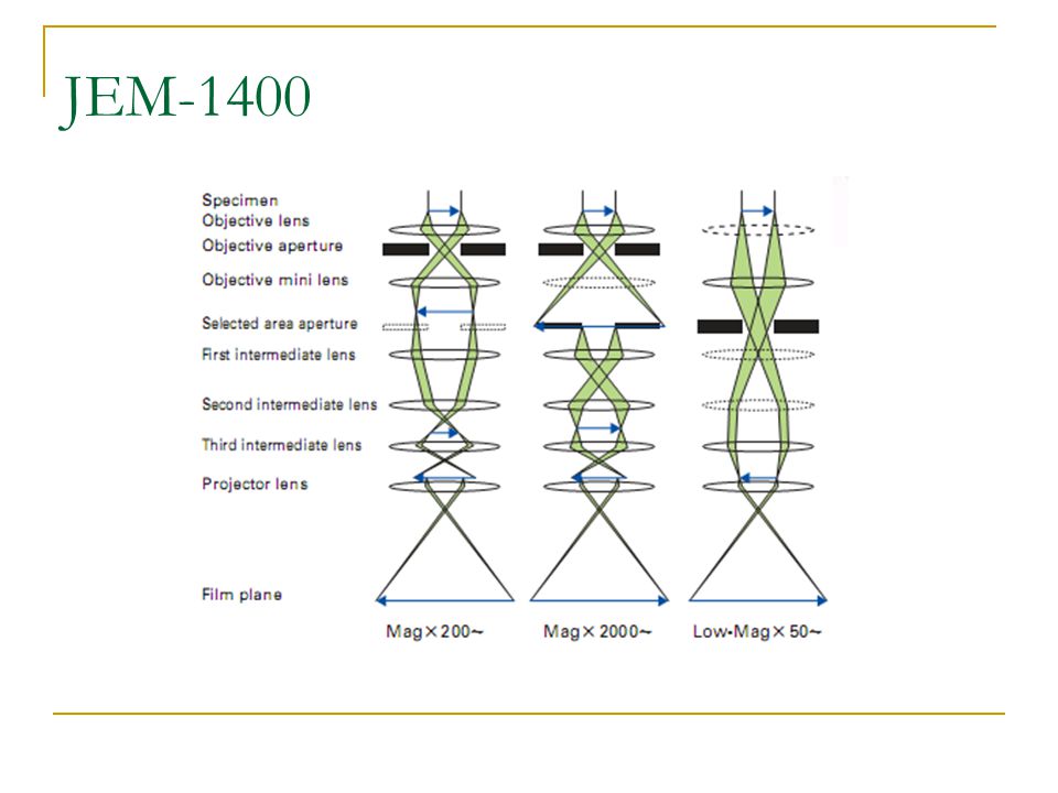
Electron microscopy www.biologie.uni-hamburg.de Confocal ImagingNonlinear TechniquesDyesEMAux JEM-1400

24
Electron microscopy Briggman, Denk, 2006 Confocal ImagingNonlinear TechniquesDyesEMAux

25
Electron microscopy. Examples. Confocal ImagingNonlinear TechniquesDyesEMAux DEMO! : rat’s brain EM sections from Kristen Harris

26
Image obtained with SEM Geological Survey of Canada, Electron Beam Laboratory

27
EM advantages and drawbacks Best resolution, available now Large depth of field Distinctive staining techniques (electron-dense (heave metal) + selective for the tissue of interest (neurons, syn) Only slices ( postmortem) Expensive Very slow Creation of the stack of images Reconstruction of the volume Confocal ImagingNonlinear TechniquesDyesEMAux
 + selective for the tissue of interest (neurons, syn) Only slices ( postmortem) Expensive Very slow Creation of the stack of images Reconstruction of the volume Confocal ImagingNonlinear TechniquesDyesEMAux")
28
END? END! Confocal ImagingNonlinear TechniquesDyesEMAux

29
Lateral resolution Defining the resolution using line-grating objects – distance between the maximum and the minimum in “Fraunhoffer slit” diffraciton. Defining the resolution using point objects – diameter of the first dark disk on the Airy diffraction image. Rayleigh criterion: the images of two equally bright spots are resolved if d ≥ r Airy (assumes that the sources radiate coherently). ? Is it true only for WF illumination? Confocal ImagingNonlinear TechniquesDyesEMAux
. Is it true only for WF illumination. Confocal ImagingNonlinear TechniquesDyesEMAux.")
30
Axial resolution Has a diffraction nature as well as the lateral resolution Thus z resolution is usually substantially larger than the xy resolution. Nevertheless don’t forget – inability to resolve objects doesn’t mean that it’s impossible to know there location Confocal ImagingNonlinear TechniquesDyesEMAux

31
Depth of field The depth of field of a microscope is the depth of the image (measured along the microscope axis translated into distances in the specimen space) that appears to be sharply in focus at one setting of the fine-focus adjustment. In bright field microscopy the depth of field should be approximately equal to the axial resolution, at least in theory. In the dark field or conventional fluorescence microscopy because of the out of focus excitation of the specimen, the depth of field is much greater than the axial resolution. In confocal imaging the depth of field correspond to the axial resolution. Moreover, it was shown using information theory (Ingelstam, 1955), that the lateral resolution becomes better by a factor of sqrt(2), when the depth of field becomes vanishingly small Confocal ImagingNonlinear TechniquesDyesEMAux
, that the lateral resolution becomes better by a factor of sqrt(2), when the depth of field becomes vanishingly small Confocal ImagingNonlinear TechniquesDyesEMAux.")
Similar presentations
 iris diaphragm.>")


 = E xo cos ( t) P x = aE xo cos ( t) + dE 2 xo cos 2 ( t) P = aE + dE 2 + d'E 3 +... Nonlinear.>")
, Phase Contrast, DIC 3.Newer.>")


