Download presentation
Presentation is loading. Please wait.

1
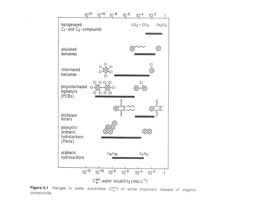
Chapter 5: Aqueous Solubility equilibrium partitioning of a compound between its pure phase and water

2
Air Water Octanol A gas is a gas is a gas T, P Fresh, salt, ground, pore T, salinity, cosolvents NOM, biological lipids, other solvents T, chemical composition Pure Phase (l) or (s) Ideal behavior PoLPoL C sat w C sat o K H = P o L /C sat w K oa KHKH K ow = C sat o /C sat w K ow K oa = C sat o /P o L
 or (s) Ideal behavior PoLPoL C sat w C sat o K H = P o L /C sat w K oa KHKH K ow = C sat o /C sat w K ow K oa = C sat o /P o L")
3
water covers 70% of the earth’s surface is in constant motion is an important vehicle for transporting chemicals through the environment Solubility is important in its own right will lead us to K ow and K aw

5
Relationship between solubility and activity coefficient Consider an organic liquid dissolving in water: for the organic liquid phase for the organic chemical in the aqueous phase at equilibrium (maximum solubility): At saturation!
: At saturation!")
6
The relationship between solubility and activity coefficient is: Assume: x iL = 1 and iL = 1 Solubility = excess free energy of solubilization (comprised of enthalpy and entropy terms) over RT or for liquids The activity coefficient is the inverse of the mole fraction solubility
 over RT or for liquids The activity coefficient is the inverse of the mole fraction solubility")
7
Solids must account for the effect of “melting” of solid i.e. additional energy is needed to melt the solid before it can be solubilized: Recall Prausnitz: At any given temperature Substitute activity coefficient for liquid solubility and rearrange: Use this for HW 5.5

8
Phase change costs or Why bother with the hypothetical liquid?

9
Melting point vs. boiling point

10
Gases solubility commonly reported at 1 bar or 1 atm (1 atm = 1.013 bar) O 2 is an exception the phase change “advantage” of condensing the gas to a liquid are already incorporated. the solubility of the hypothetical superheated liquid (which you might get from an estimation technique) may be calculated as: Actual partial pressure of the gas in your system theoretical “partial” pressure of the gas at that T (i.e. > 1 atm)
 may be calculated as: Actual partial pressure of the gas in your system theoretical partial pressure of the gas at that T (i.e. > 1 atm).")
11
concentration dependance of In reality, at saturation at infinite dilution However, for compounds with > 100 assume: at saturation = at infinite dilution i.e. solute molecules do not interact, even at saturation

12
Molecular picture of the dissolution process The two most important driving forces in determining the extent of dissolution of a substance in any liquid solvent are an increase in disorder (entropy) of the system compatability of intermolecular forces of attraction.
 of the system compatability of intermolecular forces of attraction.")
13
Ideal liquids The solubility of ideal liquids is determined by energy lowering from mixing the two substances. For ideal liquids in dilute solution in water, the intermolecular attractive forces are identical, and H mix = 0. The molar free energy of solution is: G s = G mix = -T S mix = RT ln (X f /X i ) G s, G mix = Gibbs molar free energy of solution, mixing (kJ/mol) -T S mix = Temperature Entropy of mixing (kJ/mol) R = gas law constant (8.414 J/mol-K) T = temperature (K) X f, X i = solute mole fraction concentration final, initial Note: mole fraction of solvent 1 for dilute solutions (dilute solution has solute conc <10 -3 M)
 G s, G mix = Gibbs molar free energy of solution, mixing (kJ/mol) -T S mix = Temperature Entropy of mixing (kJ/mol) R = gas law constant (8.414 J/mol-K) T = temperature (K) X f, X i = solute mole fraction concentration final, initial Note: mole fraction of solvent 1 for dilute solutions (dilute solution has solute conc <10 -3 M).")
14
solvent solute two-phase form - low disorder solution form - high disorder dissolution The greater the dilution, the smaller (i.e., more negative) the value of G s and the more spontaneous in the dissolution process
 the value of G s and the more spontaneous in the dissolution process")
15
Nonideal liquids The intermolecular attractive forces are not normally equal in magnitude between organics and water. G s G mix (no longer equal) Instead: G s = G mix + G e G e = Excess Gibbs free energy (kJ/mol) G s = H s - T S s = H e - T( S mix + S e ) H e, S e = Excess enthalpy and excess entropy (kJ/mol) H e = intermolecular attractive forces; cavity formation (solvation) S e = cavity formation (size); solvent restructuring; mixing
 Instead: G s = G mix + G e G e = Excess Gibbs free energy (kJ/mol) G s = H s - T S s = H e - T( S mix + S e ) H e, S e = Excess enthalpy and excess entropy (kJ/mol) H e = intermolecular attractive forces; cavity formation (solvation) S e = cavity formation (size); solvent restructuring; mixing.")
16
Enthalpy: For small molecules, enthalpy term is small (± 10 kJ/mol) Only for large molecules is enthalpy significant (positive) Entropy: Entropy term is generally favorable Except for large compounds, for which water forms a “flickering crystal”, which fixes both the orientation of the water and of the organic molecule
 Only for large molecules is enthalpy significant (positive) Entropy: Entropy term is generally favorable Except for large compounds, for which water forms a flickering crystal , which fixes both the orientation of the water and of the organic molecule")
17
Solubility Process A mechanistic perspective of solubilization process for organic solute in water involves the following steps: a. break up of solute-solute intermolecular bonds b. break up of solvent-solvent intermolecular bonds c. formation of cavity in solvent phase large enough to accommodate solute molecule d. vaporization of solute into cavity of solvent phase e. formation of solute-solvent intermolecular bonds f. reformation of solvent-solvent bonds with solvent restructuring

18
Estimation technique Activity coefficients and water solubilities can be estimated a priori using molecular size, through molar volume (V, cm 3 /mol). Molar volumes in cm 3 /mol can be approximated: N i = number of atoms of type i in jth molecule a i = atomic volume of ith atom in jth molecule (cm 3 /mol) n j = number of bonds in jth molecule (all types) a values: see p. 149 Solubility can approximated using a LFER of the type:
 n j = number of bonds in jth molecule (all types) a values: see p. 149 Solubility can approximated using a LFER of the type:.")
19
Molar volume here must be estimated by the atom fragment technique (see p. 149)
")
20
This type of LFER is only applicable within a group of similar compounds:

21
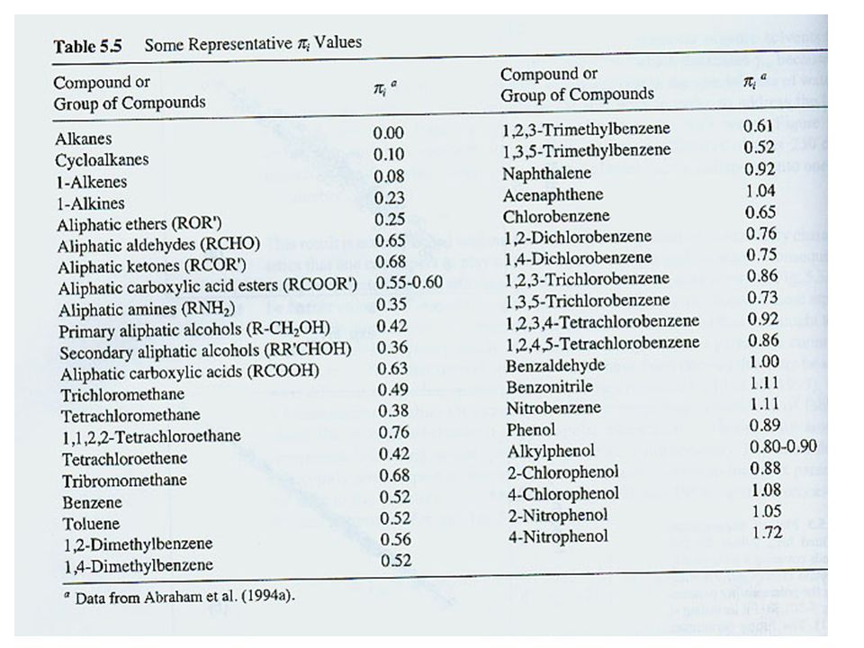
Another estimation technique Note that this is similar to the equation we used to estimate vapor pressure, but is much more complicated! Also, introduced , the polarizability term. This approach is universal – valid for all compounds/classes/types This approach can also be used (with different coefficients) to predict other physical properties (for example, solubility in solvents other than water). VP describes self:self interactions molar volume describes vdW forces refractive index describes polarity additional polarizability term H-bonding cavity term
 to predict other physical properties (for example, solubility in solvents other than water). VP describes self:self interactions molar volume describes vdW forces refractive index describes polarity additional polarizability term H-bonding cavity term.")
23
Factors Influencing Solubility in Water Temperature Salinity pH Dissolved organic matter (DOM) Co-solvents
 Co-solvents")
24
Temperature effects on solubility Generally: as T , solubility for solids. as T , solubility can or for liquids and gases. BUT For some organic compounds, the sign of H s changes; therefore, opposite temperature effects exist for the same compound! The influence of temperature on water solubility can be quantitatively described by the van't Hoff equation as: ln C sat = - H/(RT) + Const. recall from thermodynamic lecture
 + Const. recall from thermodynamic lecture.")
25
What H is this? Liquids: Solids: OR Pure liquid water gas Pure solid solid liquid aqueous gas the energy (enthalpy) needed to get the liquid (real or hypothetical) compound into aqueous solution Note: sometimes energy states are higher/lower, so some of these enthalpy terms could be negative!
 needed to get the liquid (real or hypothetical) compound into aqueous solution Note: sometimes energy states are higher/lower, so some of these enthalpy terms could be negative!.")
26
Solids, liquids, gases… Solids Liquids Gases Parameters for this plot: solid liquid gas TbTb TmTm

27
Salinity effects on solubility As salinity increases, the solubility of neutral organic compounds decreases (activity coefficient increases) K s = Setschenow salt constant (depends on the compound and the salt) [salt] = molar concentration of total salt. The addition of salt makes it more difficult for the organic compound to find a cavity to fit into, because water molecules are busy solvating the ions. typical seawater [salt] = 0.5M
![Salinity effects on solubility As salinity increases, the solubility of neutral organic compounds decreases (activity coefficient increases) K s = Setschenow salt constant (depends on the compound and the salt) [salt] = molar concentration of total salt.](http://images.slideplayer.com/18/5693422/slides/slide_27.jpg "The addition of salt makes it more difficult for the organic compound to find a cavity to fit into, because water molecules are busy solvating the ions. typical seawater [salt] = 0.5M.")
30
pH can increase apparent solubity pH effect depends on the structure of the solute. If the solute is subject to acid/base reactions then pH is vital in determining water solubility. The ionized form has much higher solubility than the neutral form. The apparent solubility is higher because it comprises both the ionized and neutral forms. The intrinsic solubility of the neutral form is not affected. We will talk about this more when we look at acid/base reactions

31
Dissolved organic matter (DOM) can increase apparent solubility DOM increases the apparent water solubility for sparingly soluble (hydrophobic) compounds. DOM serves as a site where organic compounds can partition, thereby enhancing water solubility. Solubility in water in the presence of DOM is given by the relation: C sat,DOM = C sat (1 + [DOM]K DOM ) [DOM] = concentration of DOM in water, kg/L K DOM = DOM/water partition coefficient Again, the intrinsic solubility of the compound is not affected.
 [DOM] = concentration of DOM in water, kg/L K DOM = DOM/water partition coefficient Again, the intrinsic solubility of the compound is not affected..")
32
Co-solvent effect on solubility the presence of a co-solvent can increase the solubility of hydrophobic organic chemicals co-solvents can completely change the solvation properties of “water” examples: –industrial wastewaters –“gasohol” –engineered systems for soil or groundwater remediation –HPLC

33
focus on sparingly soluble solutes completely water-miscible organic solvents –methanol, ethanol, propanol, acetone, dioxane, acetonitrile, dimethylsulfoxide, dimethylformamide, glycerol, and more What do these solvents have in common?

34
In general solubility increases exponentially as cosolvent fraction increases. need 5-10 volume % of cosolvent to see an effect. extent of solubility enhancement depends on type of cosolvent and solute –effect is greatest for large, nonpolar solutes –more “organic” cosolvents have greater effect propanol>ethanol>methanol

35
Bigger, more non-polar compounds are more affected by co-solvents Different co-solvents behave differently, behavior is not always linear We can develop linear relationships to describe the affect of co-solvents on solubility. These relationships depend on the type and size of the solute

36
Quantifying cosolvent effect can be complex, so assume log-linear relationship between solubility and volume fraction of cosolvent (f v ) if f v 1 = 0, then we are describing the solubility enhancement relative to the standard aqueous solubility: i c is the slope term, which depends on the both the cosolvent and solute
 if f v 1 = 0, then we are describing the solubility enhancement relative to the standard aqueous solubility: i c is the slope term, which depends on the both the cosolvent and solute")
37
Problem 5.4 estimate the solubilities of 1-heptene and isooctane (2,2,4 trimethylpentane) isoctane: = 0.692 g/mL 1-heptene = 0.697 g/mL Characteristic volumes: H = 8.71 C = 16.35 -per bond = 6.56
 isoctane: = g/mL 1-heptene = g/mL Characteristic volumes: H = 8.71 C = per bond = 6.56")
Similar presentations


 dissolving in water (solvent): –H-bonds in water have to be interrupted, –KCl dissociates into.>")
->")


