1. Lecture 12: Introduction to Discrete Fourier Transform Sections 2.2.3, 2.3

2. 5*sin (2  4t) Amplitude = 5 Frequency = 4 Hz seconds Review: A sine wave

3. 5*sin(2  4t) Amplitude = 5 Frequency = 4 Hz Sampling rate = 256 samples/second seconds Sampling duration = 1 second Review: A sine wave signal

4. Review: An undersampled signal

5. Review: The Nyquist Frequency The Nyquist frequency is equal to one-half of the sampling frequency. The Nyquist frequency is the highest frequency that can be measured in a signal.

6. The Fourier Transform A transform takes one function (or signal) and turns it into another function (or signal) Continuous Fourier Transform: close your eyes if you don’t like integrals

7. A transform takes one function (or signal) and turns it into another function (or signal) The Discrete Fourier Transform: The Fourier Transform

8. Fast Fourier Transform The Fast Fourier Transform (FFT) is a very efficient algorithm for performing a discrete Fourier transform FFT principle first used by Gauss in 18?? FFT algorithm published by Cooley & Tukey in 1965 In 1969, the 2048 point analysis of a seismic trace took 13 ½ hours. Using the FFT, the same task on the same machine took 2.4 seconds!

9. Famous Fourier Transforms Sine wave Delta function

10. Famous Fourier Transforms Gaussian

11. Famous Fourier Transforms Sinc function Square wave

12. Famous Fourier Transforms Sinc function Square wave

13. Famous Fourier Transforms Exponential Lorentzian

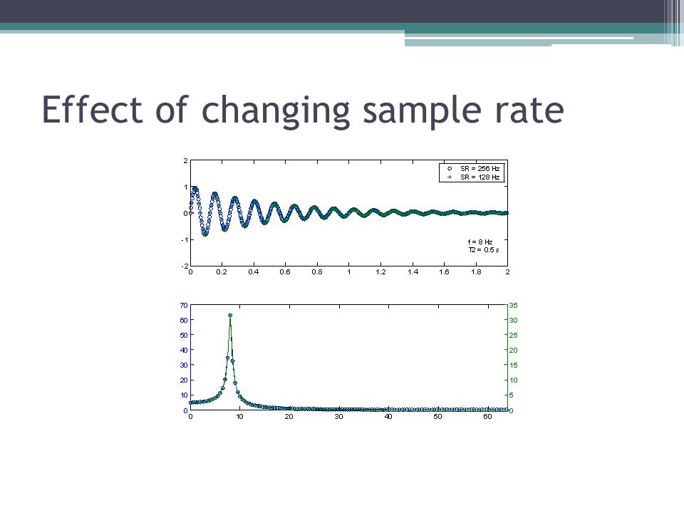
14. Effect of changing sample rate

16. Lowering the sample rate: ▫Reduces the Nyquist frequency, which ▫Reduces the maximum measurable frequency ▫Does not affect the frequency resolution

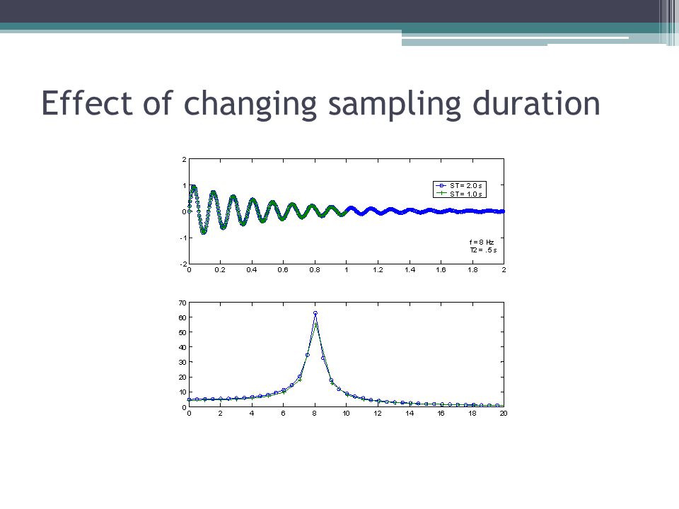
17. Effect of changing sampling duration

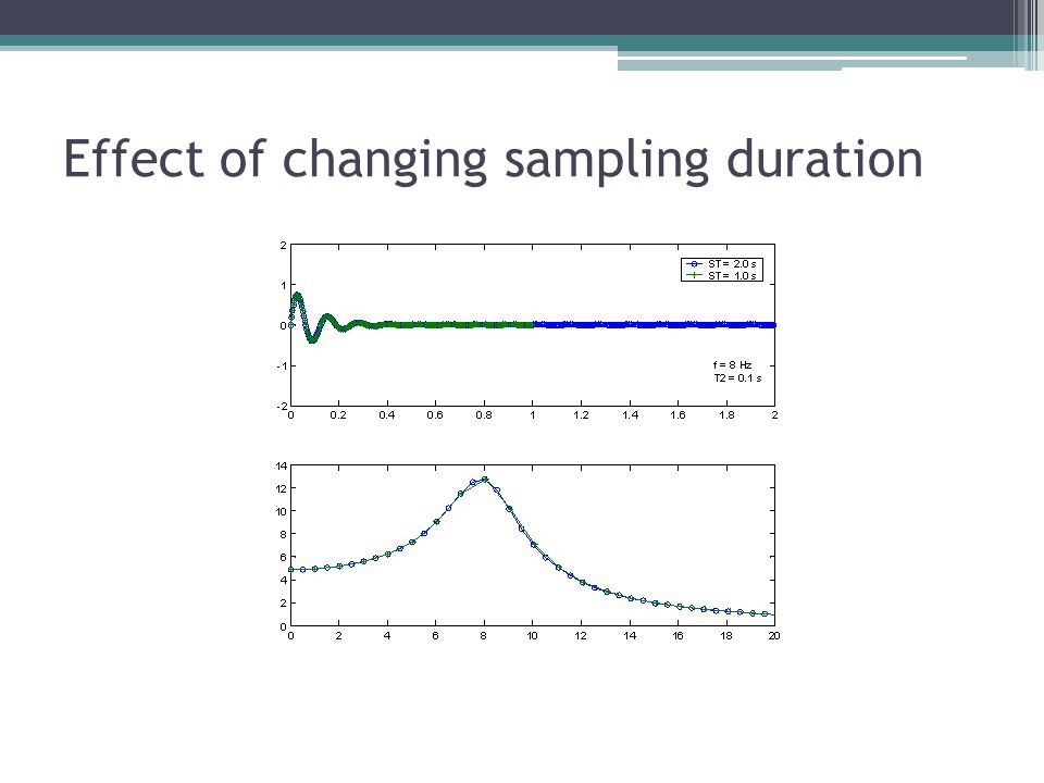
19. Reducing the sampling duration: ▫Lowers the frequency resolution ▫Does not affect the range of frequencies you can measure

20. Effect of changing sampling duration

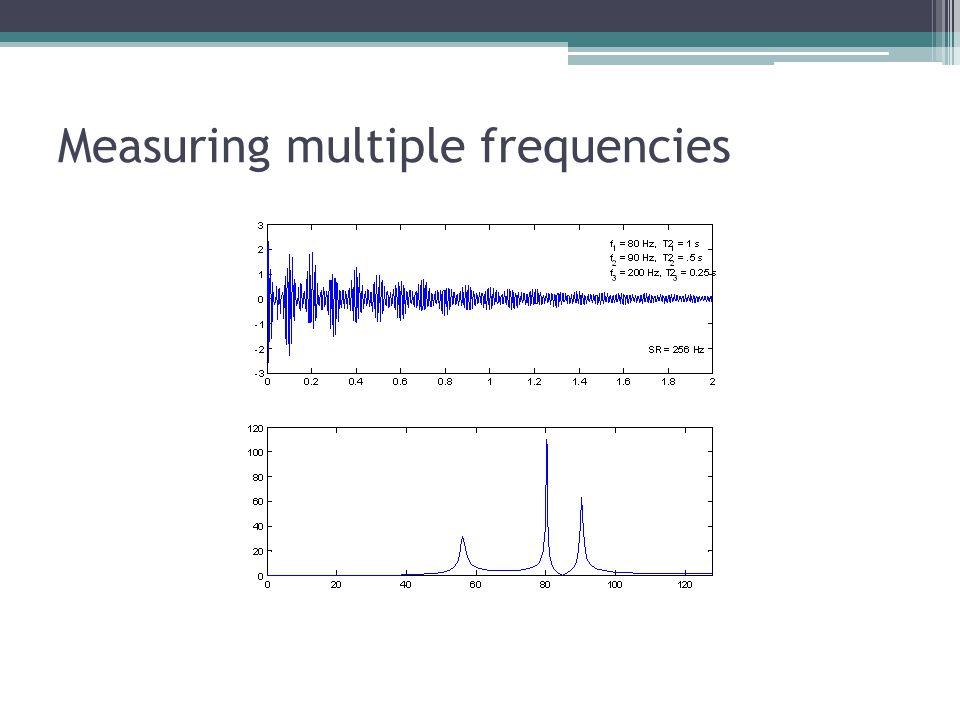
22. Measuring multiple frequencies

24. FFT in matlab Assign your time variables ▫t = [0:255]; Assign your function ▫y = cos(2*pi*n/10); Choose the number of points for the FFT (preferably a power of two) ▫N = 2048; Use the command ‘fft’ to compute the N-point FFT for your signal ▫Yf = abs(fft(y,N)); Use the ‘fftshift’ command to shift the zero-frequency component to center of spectrum for better visualization of your signals spectrum ▫Yf= fftshift(Yf); Assign your frequency variable which is your x-axis for the spectrum ▫f = [-N/2:N/2-1]/N; - this is the normalized frequency symmetrical about f 0 and about the y-axis Plot the spectrum ▫plot(f, Yf)

25. FFT in matlab Vary the sampling frequency and see what happens Vary the sample duration and see what happens

26. Spectrum of a signal