Download presentation
Presentation is loading. Please wait.

1
Simulations with MEGAlib Jau-Shian Liang Department of Physics, NTHU / SSL, UCB 2007/05/15

2
Compton Telescopes cos() = 1 - m e c 2 ( 1/E 2 - 1/E t ) E t = E 1 + E 2
 = 1 - m e c 2 ( 1/E 2 - 1/E t ) E t = E 1 + E 2")
3
The gamma-ray cross-sections for germanium (Density: 5.323 g/cm 3 )
")
4
Multiple Compton scattering The energy of this gamma ray is uniquely determined by the energy losses of the first two interactions, L 1, L 2,and 2.

5
the angular resolution measure(ARM) The angular resolution measure (ARM) is defined as the smallest angular distance between the known origin of the photon and the Compton cone.
 The angular resolution measure (ARM) is defined as the smallest angular distance between the known origin of the photon and the Compton cone.")
6
Uncertainties measuring error Measurement uncertainty of the Compton scatter angle d as a function of the Compton scatter angle . An initial energy of 2 MeV was assumed. The solid lines correspond to an error in percent of energy of the scattered gamma ray, the dotted lines to a constant error. including position error and energy error

7
incomplete absorption Doppler broadening In a real-life detector system the electrons are neither free nor at rest, but bound to a nucleus. In 1929 DuMond (1929) interpreted a measured broadening of Compton spectra as Doppler broadening induced by the velocity of the electrons.
 interpreted a measured broadening of Compton spectra as Doppler broadening induced by the velocity of the electrons..")
8
Dependence of the angular resolution on the nuclear charge. Doppler broadening as a lower limit to the angular resolution of a Compton telescope

9
Dependence of the angular resolution on the Compton scatter angle for Germanium at four energies at the Doppler-broadening limit. Dependence of the angular resolution on the energy of the initial gamma ray at the Doppler broadening limit.

10
Silicon vs. Germanium Si 1. less “ Doppler broadening ” 2. higher operating temperatures Ge 1. higher stopping power 2. energy resolution is better 3. available in larger detector volumes

11
Process Geometry & Detector information Simulation Event reconstruction & selection Back projection Image reconstruction

12
-ray simulation Extensive simulations of a Compton Telescope are performed using MGGPOD and GEANT4 Monte Carlo packages.

13
event reconstruction The permutation with the best quality factor is chosen as the correct sequence of interactions. The quality factor describes the probability that the event happened this way and is completely absorbed.

14
Back-projection of Compton circles from simulated 0.662 MeV point source. Back-projection

15
image reconstruction 10 iterations of LMEM algorithm on simulated 0.662 MeV point source.

16
geometry & trigger 8 detectors Material: Germanium Thickness: 0.6cm Strip number: 300*300 Depth resolution: 0.1cm Noise threshold: 0 Energy resolution: 0 Failure rate: 0 30 cm 21 cm

17
Sources 200 keV Point source @ =0 o, =0 o 511 keV Point source @ =0 o, =0 o 1000 keV Point source @ =0 o, =0 o 2000 keV Point source @ =0 o, =0 o 511 keV ring shape source with 20 degree radius @ =0 o, =0 o

18
Selection criteria Compton scatter angle: 0 o ~ 90 o Compton quality factor: 0 ~ 10 5 Interaction sequence length: 3 ~ 8

19
Results Effective area

20
The energy spectrum without energy recoverywith energy recovery incomplete absorption 200 keV 511 keV 200 keV 511 MeV

21
without energy recoverywith energy recovery 1 MeV 2 MeV 1 MeV 2 MeV

22
200 keV 1 MeV 511 keV 2 MeV image reconstruction

23
FWHM of ARM The histogram of ARM @ 511 keV

24
ARM vs. Compton quality factor without energy recovery with energy recovery

25
Energy vs. Compton quality factor without energy recovery with energy recovery

26
Compton sequence length vs. Compton quality factor without energy recovery with energy recovery

27
511 keV ring shape source with 20 degree radius Image reconstruction for ring shape source

28
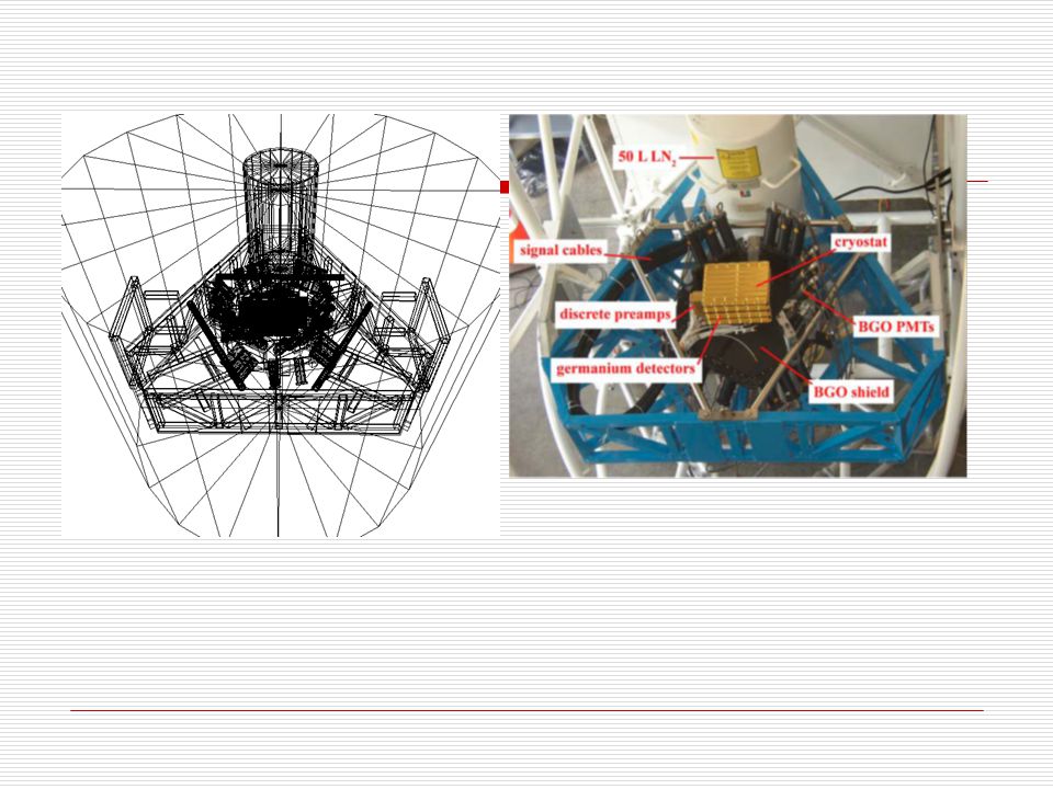
NCT model ( S. E. Boggs, CIS workshop 2005 @ NTHU )
")
30
Next steps… Complete the NCT model Background information (provided by Andreas) 511 keV line spectra and spatial distribution (provided by Gwan-Ting) To do the simulation of 511 keV line distribution Else...
 511 keV line spectra and spatial distribution (provided by Gwan-Ting) To do the simulation of 511 keV line distribution Else...")
Similar presentations


 light emitted during electronic recombination in the scintillator. Therefore, the spectrum collected.>")


