Download presentation
Presentation is loading. Please wait.

1
Systematics in the Pierre Auger Observatory Bruce Dawson University of Adelaide for the Pierre Auger Observatory Collaboration

2
Introduction Fluorescence - a technique with great rewards, but a lot of work required! Will concentrate on energy measurement (e.g. composition has an additional set of systematics) All good experiments build in CROSS-CHECKS, Auger no exception. Clearly, most important cross-check is the Hybrid nature of Auger, but many others.
 All good experiments build in CROSS-CHECKS, Auger no exception. Clearly, most important cross-check is the Hybrid nature of Auger, but many others..")
3
The Observatory Mendoza Province, Argentina 3000 km 2, 875 g cm -2 1600 water Cherenkov detectors 1.5 km grid 4 fluorescence eyes - total of 24 telescopes each with 30 o x 30 o FOV 65 km

4
Engineering Array

5
Simulated Hybrid Aperture Hybrid Trigger Efficiency “Stereo” Efficiency

6
Hybrid Reconstruction Quality 68% error bounds given detector is optimized for 10 19 eV, but good Hybrid reconstruction quality at lower energy E(eV) dir ( o ) Core (m) E/E (%) X max g/cm 2 10 18 0.7601338 10 19 0.550725 10 20 0.550624 statistical errors only zenith angles < 60 O Statistical errors only!
 dir ( o ) Core (m) E/E (%) X max g/cm statistical errors only zenith angles < 60 O Statistical errors only!")
7
Steps to good energy reconstruction Geometry Calibration: atmosphere and optical Analysis –Light collection –Cherenkov subtraction –Fitting function –Missing energy –Fluorescence yield

8
Geometry Reconstruction eye determines plane containing EAS axis and eye –plane normal vector known to an accuracy of ~ 0.2 o to extract R p and eye needs to measure angular velocity and its time derivative d /dt –but difficult to get d /dt, leads to degeneracy in (R p degeneracy broken with measurement of shower front arrival time at one or more points on the ground –eg at SD water tank positions

9
Geometry Reconstruction Simulations at 10 19 eV Reconstruct impact parameter Rp. Dramatic improvement with Hybrid reconstruction Single FD only median R p error = 350m strong dependence on angular “Track Length” Hybrid median Rp error = 20 m (Will check with stereo events)
.")
10
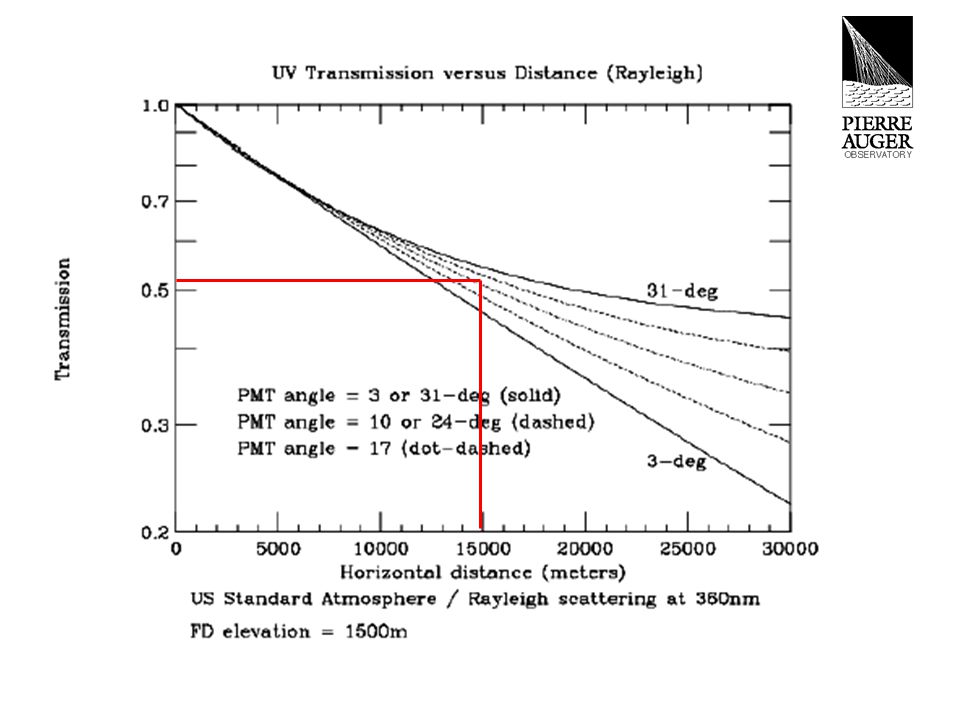
Atmosphere Systematics light transmission corrections (Rayleigh and aerosol scattering) AIM: know corrections to better than 10% air density profile with height (mapping height to depth; Rayleigh scattering) AIM: know overburden at a given height to better than 15 g/cm 2
 AIM: know corrections to better than 10% air density profile with height (mapping height to depth; Rayleigh scattering) AIM: know overburden at a given height to better than 15 g/cm 2")
11
Distance from pixels to track MC: 10 19 eV events over full array Closest triggering eye

13
VARIABLE !!

14
Horizontal attenuation monitors (50km) Steerable LIDARs - total optical depth Vertical lasers near centre of array - vertical distribution of aerosols Cross-checks
 Steerable LIDARs - total optical depth Vertical lasers near centre of array - vertical distribution of aerosols Cross-checks")
15
Aerosol measurements (John Matthews ICRC 2001)
")
16
LIDAR System

17
Tests near Torino System at Los Leones

18
Some simulations Simulations: 1000 10 19 eV showers landing within Auger full array. Generate with fixed aerosol parameters: –horizontal attenuation length (334nm) al = 25 km –scale height of aerosol layer ha = 1.0 km –height of “mixing layer” hm = 0 km First, reconstruct events with different aerosol assumptions
 al = 25 km –scale height of aerosol layer ha = 1.0 km –height of mixing layer hm = 0 km First, reconstruct events with different aerosol assumptions.")
19
Dependence on Aerosol Parameters (generated with al=25km, ha=1.0km, hm=0km) reconstruct with 19km 1.0km 0km E/E = +8% X max = +7 g/cm 2 reconstruct with 40km 1.0km 0km E/E = -9% X max = -9 g/cm 2 reconstruct with 25km 2.0km 0km E/E = +10% X max = -2 g/cm 2 reconstruct with 25km 1.0km 0.5km E/E = +12% X max = +8 g/cm 2
 reconstruct with 19km 1.0km 0km E/E = +8% X max = +7 g/cm 2 reconstruct with 40km 1.0km 0km E/E = -9% X max = -9 g/cm 2 reconstruct with 25km 2.0km 0km E/E = +10% X max = -2 g/cm 2 reconstruct with 25km 1.0km 0.5km E/E = +12% X max = +8 g/cm 2")
20
Atmosphere Density Profile Density profile of atmosphere determines mapping from height to depth, and Rayleigh scattering MC generated with vertical overburden 873 g/cm 2 and one of the US Standard Atmospheres. Will maintain scale height. reconstruct with vertical overburden 900 g/cm 2 E/E = +2.2% X max = +19 g/cm 2 reconstruct with vertical overburden 845 g/cm 2 E/E = - 3.3% X max = - 19 g/cm 2

21
Radiosonde Balloon-borne radiosondes are planned to monitor the atmosphere’s density and temperature profile First flight in August 2002 at Malargue. A series of flights in the austral spring, summer, winter and autumn will determine the suitability of re-scaled “standard atmospheres”, and variability.

22
Optical Calibration

24
Drum Calibration 375nm LEDs NIST calibrated Silicon detector uniformly illuminates aperture with full range of incoming angles in future will also use range of colours absolute calib to 7% now, hope to improve to 5%

25
Relative calibration Xenon

27
Laser shots at 3km - cross check on absolute calibration … and also are checking with piece by piece calibration.

28
Reconstruction

29
installed at Los Leones (Malargüe) and taking data corrector lens camera 440 PMTs 11 m 2 mirror UV-Filter 300-400 nm
 and taking data corrector lens camera 440 PMTs 11 m 2 mirror UV-Filter nm")
30
No coma, good light collection

31
Hybrid event. Dec 2001- March 2002

32
Light Flux at Camera Aim: to collect all signal without too much noise or multiple scattered light. Effect of multiple scattered light? Halo? currently a 10-15% systematic, is being studied optical spot 0.5 deg diam

33
time (100ns bins) photons (equiv 370nm) Estimate of Cherenkov contamination Total F(t) direct Rayleigh aerosol REAL event
 photons (equiv 370nm) Estimate of Cherenkov contamination Total F(t) direct Rayleigh aerosol REAL event")
34
Dependence on Cherenkov Yield MC generated with nominal Cherenkov yield (easy calculation if you know the density profile of atmosphere and the energy spectrum of electrons) reconstruct with Cherenkov yield up by 30% E/E = - 4.8% X max = - 9 g/cm 2 reconstruct with Cherenkov yield reduced by 30% E/E = + 5.3% X max = +9 g/cm 2 (These are averages. Clearly, the error for each event depends on its geometry).
..")
35
CORSIKA Check

36
Cherenkov correction clearly depends on more than yield calculation, also… –atmospheric scattering –geometry important problem that needs study, since all events have some contamination stereo will be an important aid

37
PRELIMINARY shower size (arb units)
")
38
PRELIMINARY shower size (arb units)
")
39
Profile T. Abu-Zayyad et al Astropart. Phys. 16, 1 (2001)
")
40
“Missing energy” correction unavoidable 5% systematic currently being checked with new CORSIKA E cal = calorimetric energy E 0 = true energy from C.Song et al. Astropart Phys (2000)
.")
41
Conclusion can’t provide an error budget now - many of the systematics are under study, and we need real (stereo) data to study many of them have indicated our goals in terms of two major players - the atmosphere (10%) and optical calibration (5%). These must be obtained early. cross-checks are vital then there is the fluorescence yield…

Similar presentations


 for the Auger.>")


 ● Atmospheric profile ( stdz76, radiosonde) ● Rayleigh Scattering ● Aerosols Model ( density, variability.>")
 Advisor: Stefan Westerhoff.>")


 By: Rasha Usama Abbasi.>")


 Collaboration GZK-40. INR, Moscow. May 17, 2006. measurements by fluorescence.>")