Download presentation
Presentation is loading. Please wait.

1
Flattening via Multi- Dimensional Scaling Ron Kimmel www.cs.technion.ac.il/~ron Computer Science Department Geometric Image Processing Lab Technion-Israel Institute of Technology

2
qOn isometric surfaces and bending invariant signatures. qMulti-dimensional scaling techniques: uClassical. uLeast squares. uFast. qSurface classification: experimental results. Outline

3
Matching Surfaces qProblem: Given 2D surfaces, define a measure of their similarity. qClassical techniques: uFind a rigid transformation that maximizes some measure. uMatch key points on the surface. uCompare local or semi-differential invariants, e.g. matching graphs.

4
qIsometric surface matching via bending invariant signatures: uMap the surface into a small Euclidean space, in which isometric surfaces transform to similar (rigid) surfaces. qAdvantages: uHandle (somewhat) non-rigid objects. uA global operation, does not rely on selected key points or local invariants. Bending Invariant Signatures
 non-rigid objects. uA global operation, does not rely on selected key points or local invariants. Bending Invariant Signatures.")
5
Bending invariant signatures Basic Concept Input – a surface in 3D Extract from [D] coordinates in an m dimensional Euclidean space via Multi-Dimensional Scaling (MDS). Output – A 2D surface embedded in in R (for some small m) i j ij Compute geodesic distance matrix [D] between each pair of vertices δ = geodesic_distance(vertex,vertex ) [D] = δ m
![Bending invariant signatures Basic Concept Input – a surface in 3D Extract from [D] coordinates in an m dimensional Euclidean space via Multi-Dimensional Scaling (MDS).](http://images.slideplayer.com/16/5195906/slides/slide_5.jpg "Output – A 2D surface embedded in in R (for some small m) i j ij Compute geodesic distance matrix [D] between each pair of vertices δ = geodesic_distance(vertex,vertex ) [D] = δ m.")
6
Fast Marching on Surfaces Source point Euclidean Distance Geodesic Distance

7
Multi-Dimensional Scaling qMDS is a family of methods that map similarity measurements among objects, to points in a small dimensional Euclidean space. qThe graphic display of the similarity measurements provided by MDS enables to explore the geometric structure of the data. Stress = Σ( δ - d ) ij 2 ΣδΣδ MDS Dissimilarity measures coordinates in m-dimensional Euclidean Space Stress Function
 ij 2 ΣδΣδ MDS Dissimilarity measures coordinates in m-dimensional Euclidean Space Stress Function.")
8
A simple example 12345678910 1. London0 2. Stockholm5690 3. Lisbon66712120 4. Madrid53010432010 5. Paris1416175964310 6. Amsterdam1404467686081770 7. Berlin3573259237403402180 8. Prague3964238826903372721140 9. Rome5697877145164365194723640 10. Dublin1906487146223203025145737550 12345678910 12.7032.829.414.68.84.56.416.413.8 4.113.913.214.99.08.216.619.625.40 x Y Stockholm London Dublin Lisbon Amsterdam Paris Prague Berlin Rome Madrid Stockholm London Dublin Lisbon Amsterdam Paris Prague Berlin Rome Madrid Stockholm London Dublin Lisbon Amsterdam Paris Prague Berlin Rome Madrid Rotation Reflection

9
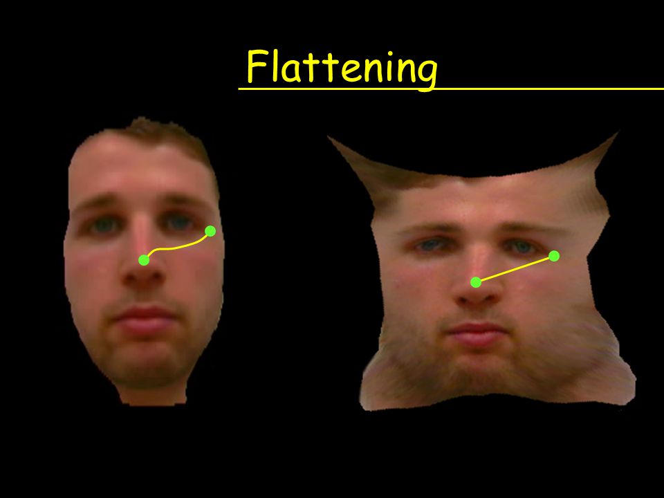
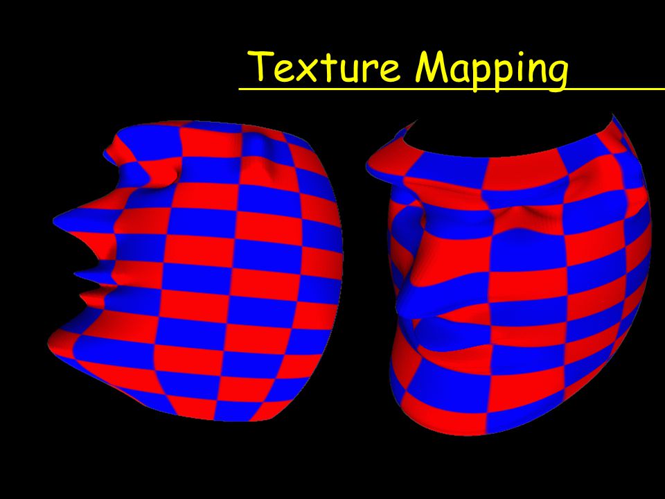
Flattening via MDS qCompute geodesic distances between pairs of points. qConstruct a square distance matrix of geodesic distances^2. qFind the coordinates in the plane via multi- dimensional scaling. The simplest is `classical scaling’. qUse the flattened coordinates for utexturing the surface, while preserving the texture features. Zigelman, Kimmel, Kiryati, IEEE TVCG 2002 Grossmann, Kiryati, Kimmel, IEEE TPAMI 2002 uBending invariant surface matching Elad (Elbaz), Kimmel CVPR 2001 0 0 0
, Kimmel CVPR")
10
Flattening

12
Distances - comparison

13
Texture Mapping

15
Fattening via MDS: 3D Original Fast Classical Least Squares Original Fast Least Squares Classical

16
Fattening via MDS: 3D Original Fast Classical Least Squares Original Fast Least Squares Classical

17
Input Surfaces

18
Bending Invariant Signatures Elad, Kimmel, CVPR’2001 ?

19
Bending Invariant Signatures ? Elad, Kimmel, CVPR’2001

20
Bending Invariant Signatures ? Elad, Kimmel, CVPR’2001

21
Bending Invariant Signatures Elad, Kimmel, CVPR’2001

22
Bending Invariant Signatures Elad, Kimmel, CVPR’2001

23
Bending Invariant Signatures 3 Original surfaces Canonical surfaces in R Elad, Kimmel, CVPR’2001

24
0 0.2 0.4 0.6 0.8 1 0 0.2 0.4 0.6 0.8 1 0 0.1 0.2 0.3 0.4 0.5 0.6 0.7 0.8 CC C C A A A A D DD D B B B B E E E E F F F F 0 0.2 0.4 0.6 0.8 1 0 0.2 0.4 0.6 0.8 1 0 0.1 0.2 0.3 0.4 0.5 0.6 0.7 0.8 C E C C B A D E E E B C A B D B F D A D F A F F Bending Invariant Clustering q2 nd moments based MDS for clustering Original surfaces Canonical forms *A=human body *B=hand *C=paper *D=hat *E=dog *F=giraffe Elad, Kimmel, CVPR’2001

25
Classical Scaling Young et al. 1930 Given n points in, denote Define coordinates vector The Euclidean distance between 2 points:

26
Define the `centering’ matrix where Let the matrix We have that and also Thus, Classical Scaling

27
The coordinates are related to by Thus the operation is also called `double centering’. Applying SVD, we can compute where and the coordinates can be extracted as If we choose to take only part of the eignstructure, then, our approximation minimizes the Frobenius norm

28
MDS Matlab code for 2D flattening Zigelman, Kimmel, Kiryati IEEE TVCG 2002

29
Classical Scaling The eigenvalues are the 2 nd order moments of the flattened surface, since by definition all the cross 2 nd order moments vanish by the unitarity of U, thus `flattening’.

30
Conclusions qA method for bending invariant signatures qBased on: uFast marching on surfaces uMDS LS/Classical/Fast uResults: uTexture mapping uBending invariant signatures uClassification of isometric surfaces.

31
Least Squares MDS qStandard optimization approach to solve the minimization problem of the stress cost function. qSolved via ‘scaling by maximizing convex function’ (SAMCOF) algorithm. qStarting with a random solution and iteratively minimizing another stress function, which satisfies. ƒ (x,z) ≥ ƒ (x) for x ≠ z and ƒ (z,z) = ƒ (z) qThe complexity is O(n ). qConverges to the optimal solution. 2
 algorithm. qStarting with a random solution and iteratively minimizing another stress function, which satisfies. ƒ (x,z) ≥ ƒ (x) for x ≠ z and ƒ (z,z) = ƒ (z) qThe complexity is O(n ). qConverges to the optimal solution. 2.")
32
Fast MDS qThe fast MDS: heuristic efficient technique O(mn). qWorks recursively by generating a new dimension at each step, Providing m-dimensional coordinates after m recursion steps. qProject the vertices on a selected ‘line’. uFirst, the algorithm selects the Farthest two vertices. uNext, all other vertices are projected On that line using the cosine law. uNext step is to project all items to An (n-1) hyper plane (H) that is Perpendicular to the line that Connects those vertices. uGenerate a new distance matrix. uRepeat the last three steps m times.
 hyper plane (H) that is Perpendicular to the line that Connects those vertices. uGenerate a new distance matrix. uRepeat the last three steps m times..")
Similar presentations
 and g() such that the images are best.>")


 Dimensionality Reductions or data projections Random projections.>")


 Given an image find.>")


 – FastMap Dimensionality Reductions or data projections.>")


 – FastMap Dimensionality Reductions or data projections.>")

