1. Seminar on Geometric Approximation Algorithms Speaker: Alon Horowitz

2. What is WSPD How to construct and represent WSPD efficiently Applications of WSPD Outline of this lecture

3. What is WSPD Let P be a set of n points in R d, and ¼ > ɛ > 0 a parameter. Say we want to represent all distances between points of P. Return all pairwise distances Return all n points in P (of size dn)

4. p q s We are interested in a representation that will capture the structure of the distances between the points. ≈ Close together as far as p is concerned As such, if we are interested in the closest pair among the three points, we will want to only check the distance between q and s.

5. Example: {1,2,3} {1,2,3} = {{1,2},{1,3},{2,3}} Denote by the set of all the (unordered) pairs of points formed by the sets A and B. We will be informal and refer to as a pair of sets A and B. Definitions

6. For a point set P, a pair decomposition of P is a set of pairs such that: 1.A i, B i P for every i 2.A i ∩ B i = ɸ for every i 3. Translation: For any pair of distinct points p,q ϵ P, there is at least one pair {A i,B i } ϵ such that p ϵ A i and q ϵ B i

7. Definitions The pair Q and R is (1/ɛ)-separated if: Max(diam(Q),diam(R)) ≤ ɛ∙d(Q,R) Where d(Q,R) = min qϵQ,sϵR Max{, } = 1/ɛ Min size ball 1/ɛ

8. Returning to the previous example: p q s The pairs {p} {q,s} and {q} {s} are 3-separated. We replaced the distance description made out of three pairs of points by distance between two pairs of sets.

9. Definitions For a point set P, a well-separated pair decomposition (WSPD) of P with parameter 1/ɛ is a pair decomposition of P with a set of pairs: such that, for any i, the sets A i and B i are 1/ɛ-separated. In the last example we got: = { {{p},{q,s}}, {{q},{s}} }

10. How to construct and represent WSPD efficiently Representation Construction algorithm Analysis

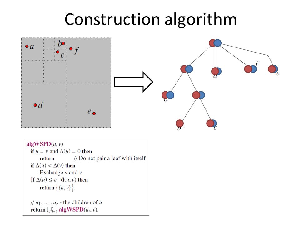
11. Representation Instead of maintaining such decomposition explicitly, it is convenient to construct a tree T having the points of P as leaves. Now every pair (A i, B i ) is just a pair of nodes (v, u) of T, such that A i = P v and B i = P u, where P v denotes the points of P stored in the subtree of v. V u (A i, B i ) = (P v, P u ) = ({b,c}, {e}) P = {a,b,c,d,e,f}

12. In our case, the tree we would use is a compressed quadtree of P. Representation There are many possible WSPDs that can be represented using the tree. We will try to find a WSPD that is “minimal”. The diameter of a point set stored in a node drops quickly

13. Construction algorithm Given a point set P in R d : Compute the compressed quadtree T of P. Greedy – tries to put into the WSPD pairs of nodes in the tree that are as high as possible: – Start from root (The pair {root,root}). – Check if current pair is well separated. – If not, replace the bigger node (diameter wise) with his children.

14. Some definitions □ v := The quadtree cell associated with the node v Δ(v) := diam(□ v ) Δ(v) = 0 if P v is either empty or a single point d(u,v) := d(□ u,□ v ) = min pϵ□ u, qϵ□ v V □v□v x d(□ v,□ f ) =d(v,f) = d(b,f) 0

15. Construction algorithm

17. 2-WSPD

18. Analysis algWSPD terminates algWSPD Computes a valid pair-decomposition The computed pairs are (1/ɛ)-separated The number of computed pairs is O(n/ɛ d ) (1/ɛ)-WSPD construction time is O(nlogn + n/ɛ d )

19. algWSPD terminates If u, v are leaves then Δ(u) = 0 and Δ(v) = 0 Δ(u) ≤ ɛ∙d(u,v)  True Always stops if both u and v are leafs Always terminates

20. algWSPD Computes a valid pair-decomposition 1. For every i, A i,B i corresponds to some P u,P v and by definition P u,P v P. 3. Every pair of points of P is covered by a pair of subsets {P u,P v } output by the algWSPD algorithm  By induction… Reminder: For a point set P, a pair decomposition of P is a set of pairs such that: 1.A i, B i P for every i 2.A i ∩ B i = ɸ for every i 3.

21. 2. Let {u,v} be an output pair If P u and P v are single point, then P u ϶ x ≠ y ϵ P v because of the first line in algWSPD  P u ∩P v =ɸ If P u or P v are not single point, then: a:= max(diam(P u ),diam(P v )) > 0 This implies that: d(P u, P v ) ≥ d(□ u,□ v ) = d(u,v) ≥ Δ(u)/ɛ ≥ a/ɛ > 0  P u ∩P v =ɸ algWSPD Computes a valid pair-decomposition

22. The computed pairs are (1/ɛ)-separated Proof: for every output pair {u,v}, we have by the design of the algorithm that: Max(diam(P u ),diam(P v )) ≤ max{Δ(u),Δ(v)} ≤ ɛ∙d(u,v) Also, for any qϵP u and sϵP v we have: d(u,v) = d(□ u,□ v ) ≤ d(P u,P v ) ≤ d(q,s) since P u □ u and P v □ v Reminder: The pair Q and R is (1/ɛ)-separated if: Max(diam(Q),diam(R)) ≤ ɛ∙d(Q,R) Where d(Q,R) = min qϵQ,sϵR

23. The number of computed pairs is O(n/ɛ d ) First, a short Lemma: Let □ be a cell of a grid G of R d with cell diameter x. For y ≥ x, the number of cells in G at distance at most y from □ is O((y/x) d ). Proof: by figure: x y+1 d = 2 O(([2(y+1)+x]/x) 2 ) = O((y/x) 2 ) In d dimensions: O((y/x) d )

24. Proof: Let {u,v} be a pair appearing in the output Let's consider the sequence of recursive calls that led to this output. In particular, Let's assume that the last recursive call to algWSPD(u,v) was issued by algWSPD(u,v’), where v’ = p(v) (the parent of v in T) This implies that Δ(u) ≤ Δ(v’) Furthermore, the fact that algWSPD(u,v’) was invoked implies that algWSPD(p(u),a(v’)) has been considered and then p(u) was split. This implies that Δ(a(v’)) ≤ Δ(p(u)) To summarize: Δ(u) ≤ Δ(v’) ≤ Δ(a(v’)) ≤ Δ(p(u)) The number of computed pairs is O(n/ɛ d )

25. Let us prove that each node v’ is charged at most O(1/ɛ d ) times Since the pair {u,v’} was not output by algWSPD (despite being considered), we conclude: Δ(v’) > ɛ∙d(u,v)  d(u,v) < Δ(v’)/ɛ := r Because we proved: Δ(u) ≤ Δ(v’) ≤ Δ(p(u)) then there are 3 possibilities: – Δ(u) = Δ(v’) – Δ(v’) = Δ(p(u)) – Δ(u) < Δ(v’) < Δ(p(u)) The number of computed pairs is O(n/ɛ d ) Possible?

26. Δ(u) = Δ(v’): by the lemma we proved, the number of u nodes that: Δ(u) = Δ(v’) and d(u,v’) < Δ(v’)/ɛ := r is at most O((r/ Δ(v’)) d ) = O(1/ɛ d ). The number of computed pairs is O(n/ɛ d ) x y+1 Since v’ has at most 2 d children, this type of charge can happen at most O(2 d ∙(1/ɛ d ))

27. Δ(v’) = Δ(p(u)): by the same argument, the number of p(u) nodes that: d(p(u),v’) ≤ d(u,v’) < r is at most O(1/ɛ d ). Since also p(u) has at most 2 d children  at most O(2 d ∙2 d ∙(1/ɛ d )) Δ(u) < Δ(v’) < Δ(p(u)): Let □’ be the cell in G containing □ u. Observe that □ u □’ □ p(u). In addition: d(□’,□ v’ ) ≤ d(□ u,□ v’ ) = d(u,v’) < r. The number of computed pairs is O(n/ɛ d ) □ p(u) □u□u □ v’ □’ As before, it follows that there are at most O(1/ɛ d ) cells like □’, and as before, total number of charges is at most O(2 d ∙(1/ɛ d )).

28. In conclusion, v’ can be charged at most O(2 d ∙2 d ∙(1/ɛ d )) = O(1/ɛ d ) times. Since there are O(n) nodes in T, the total number of pairs generated by algWSPD is O(n/ɛ d ). The number of computed pairs is O(n/ɛ d ) Every point of P is present in O(1/ɛ d ) pairs. Since running time of algWSPD is linear in the output size, and quadtree construction time is O(nlogn) we conclude: (1/ɛ)-WSPD construction time is O(nlogn + n/ɛ d )

29. Applications of WSPD Closest pair All nearest neighbors Spanners Approximating the Minimum Spanning Tree

30. Closest pair Let P be a set of points in R d, we would like to compute the closest pair. Lemma: let W be a (1/ɛ)-WSPD of P, for ɛ ≤ ½. There exists a pair {u,v}ϵW, such that: – |P u | = |P v | = 1 – is the distance of the closest pair.

31. Proof: Let p,q be the closest pair and let {u,v}ϵW be the pair such that pϵP u and qϵP v Let assume by contradiction that there is an additional point sϵ P u Closest pair Contradiction to p,q being the closest pair

32. Algorithm: Compute 2-WSPD of P Scan all pairs of W Compute distance between pairs {u,v} which are singletons Return the closest pair encountered Closest pair

33. Given a set P of points in R d, we would like to compute for each point qϵP its nearest neighbor in P. Is nearest neighbor a symmetrical relationship? All nearest neighbors q is the nearest neighbor to p, but s is the nearest neighbor to q

34. All nearest neighbors Algorithm: Compute 4-WSPD of P Scan all pairs of W Compute distance between pairs {u,v} such that P u or P v is a singleton For each P u = {p}, record for p the closest point to it in P v Return the recorded nearest point for every point p in P

35. Lemma: Let p be a point in P and let q be the nearest neighbor to p in P\{p}, then there exists a pair {u,v}ϵW such that P u ={p} and qϵP v Proof: Consider {u,v}ϵW such that pϵP u and qϵP v All nearest neighbors If P u contained any other point except p then contradiction to q being the nearest neighbor to p Diam(P u ) ≤ ɛd(P u, P v ) ≤ ɛ||p-q|| ≤ ||p-q||/4

36. Let P be a set of n points in the plane, then one can solve the all nearest neighbor problem, in O(n(logn + logɸ(P)) time, where ɸ is the spread of P All nearest neighbors Difficulties: according to the algorithm:  Compute distance between pairs {u,v} such that P u or P v is a singleton  For each P u = {p}, record for p the closest point to it in P v What if P v is very big???

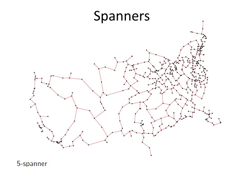
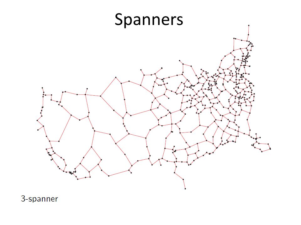
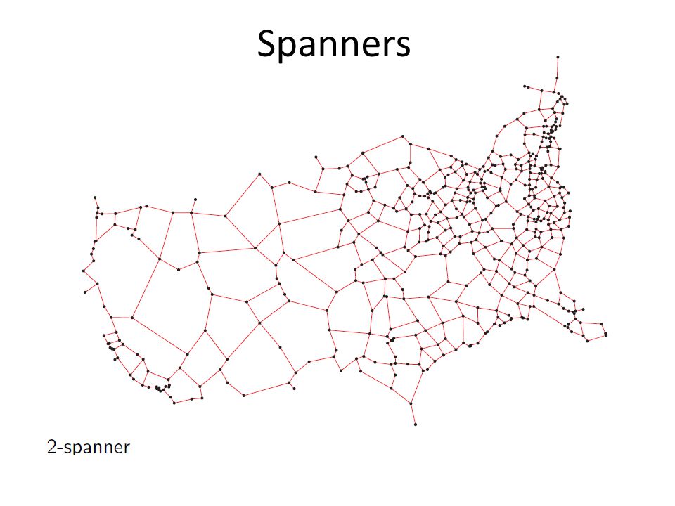
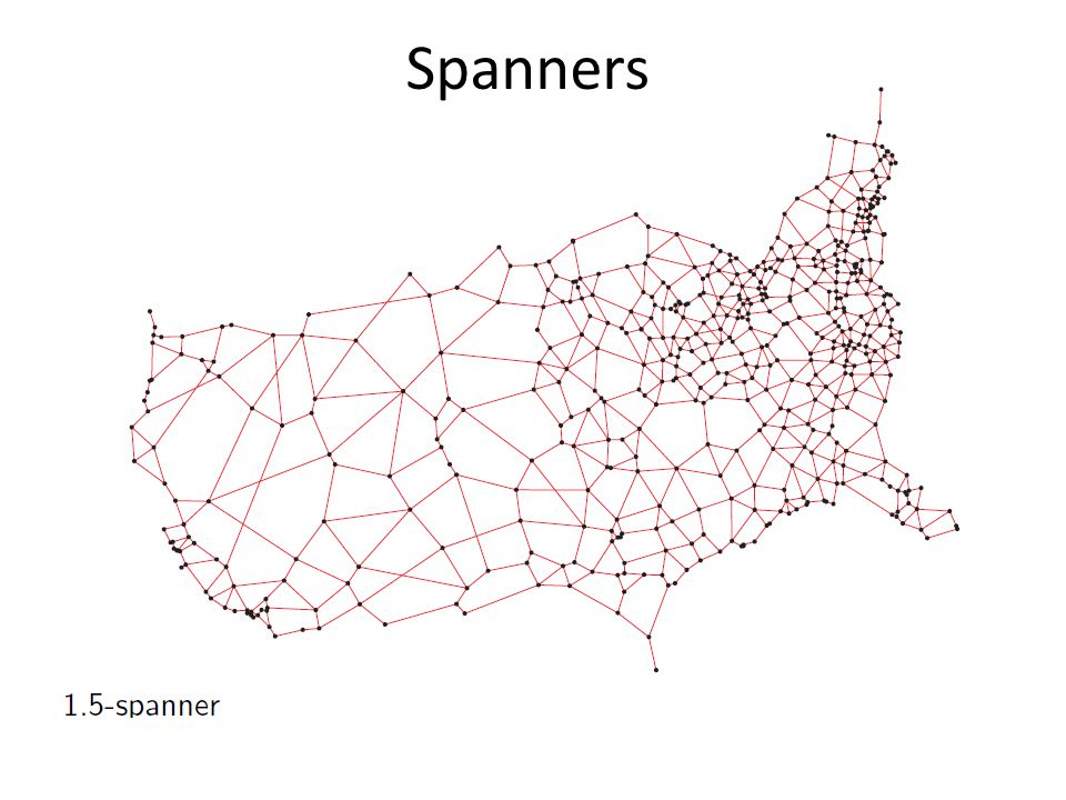
37. Spanners Definitions: d G (q,s) := distance of the shortest path between vertices q,s in weighted graph G. A t-spanner of a set of points P in R d is a weighted graph G whose vertices are the points of P, and for any q,sϵP, we have:  d G is a metric (complies with the triangle inequality)

38. Let P be a set of n points in R d and let 1 ≥ ɛ > 0 be a parameter we would like to compute a (1+ɛ)-spanner of P with O(n/ɛ d ) edges in O(nlogn + n/ɛ d ) time Spanners (1+ɛ)-spanners approximate the complete graph with a relative error ɛ

39. Spanners

44. Algorithm: Set δ = ɛ/c, where c ≥ 16 Compute a (1/δ)-WSPD of P For every pair {u,v}ϵW, add an edge between {rep u, rep v } with weight Spanners Return resulting graph G

45. Analysis: We will show that for any pair x,yϵP: – ||x-y|| ≤ d G (x,y) – d G (x,y) ≤ (1+ɛ)||x-y|| Proof: ||x-y|| ≤ d G (x,y) is trivial… why? Triangle inequality Spanners ||x-y|| d G (x,y)

46. d G (x,y) ≤ t||x-y|| by induction on the distance of the pairs: Let's assume that for any pair z,wϵP: ||z-w||<||x-y||  d G (z,w) ≤ (1+ɛ)||z-w|| The pair x,y must appear in some pair {u,v}ϵW, where xϵP u and yϵP v, thus: (*) Spanners Also: (**)

47. We conclude: d G (x,y) ≤ d G (x,rep u ) + d G (rep u,rep v ) + d G (rep v,y) ≤ (1+ɛ)∙||rep u -x|| + d G (rep u,rep v ) + (1+ɛ)∙||rep v -y|| = (1+ɛ)∙||rep u -x|| + ||rep u -rep v || + (1+ɛ)∙||rep v -y|| ≤ 2 (1+ɛ)δ∙||rep u -rep v || + ||rep u -rep v || ≤ (1+2δ+2ɛδ)∙||rep u -rep v || ≤ (1+2δ+2ɛδ)(1+2δ)∙||x-y|| ≤ (1+ɛ)∙||x-y|| Spanners (*) δ = ɛ/c and c ≥ 16 (**) (rep u,rep v ) Is an edge Induction hypothesis

48. Approximating the Minimum Spanning Tree Given a set P of n points in R d, we would like to compute a spanning tree T of P such that: w(T) ≤ (1+ɛ)w(M) where M is the minimum spanning tree of P, and w(T) is the total weight of the edges of T.

49. Approximating the Minimum Spanning Tree Algorithm: Compute a (1+ɛ)-spanner G of P Compute the minimum spanning tree T of G Return T as the approximate minimum spanning tree Running Time: Computing a minimum spanning tree of a graph, with n vertices and m edges takes O(nlogn + m) time  Computing T takes O(nlogn + n/ɛ d ) time

50. We need to prove that T is the required approximation Proof: π(q,s) : = shortest path between q and s in G M:= the minimum spanning tree of P Since G is a (1+ɛ)-spanner, for any q,sϵP: w(π(q,s)) ≤ (1+ɛ)||q-s|| Let’s look at G’ = (P,E) which is a connected subgraph of G, where E = Approximating the Minimum Spanning Tree

51. Since G is a (1+ɛ)-spanner: Since G’ is a connected spanning subgraph of G: w(T) ≤ w(G’) ≤ (1+ɛ)w(M) Approximating the Minimum Spanning Tree

52. 100 points On a Circle