Download presentation
Presentation is loading. Please wait.

1
Stata Review: Part II Biost/Epi 536 Discussion Section October 13, 2009

2
Indicator (Dummy) Variables Created from an existing categorical variable (e.g., bmicat ) Assigned value of 0 or 1 1, if the condition is true 0, if the condition is false ------------------------------------------------------------------- bmicat BMI (categorical) ------------------------------------------------------------------- type: numeric (float) label: bmicat_label range: [0,3] units: 1 unique values: 4 missing.: 5/60 tabulation: Freq. Numeric Label 10 0 Underweight 17 1 Normal 17 2 Overweight 11 3 Obese 5.
![Indicator (Dummy) Variables Created from an existing categorical variable (e.g., bmicat ) Assigned value of 0 or 1 1, if the condition is true 0, if the condition is false bmicat BMI (categorical) type: numeric (float) label: bmicat_label range: [0,3] units: 1 unique values: 4 missing.: 5/60 tabulation: Freq.](http://images.slideplayer.com/16/5121916/slides/slide_2.jpg "Numeric Label 10 0 Underweight 17 1 Normal 17 2 Overweight 11 3 Obese 5..")
3
Indicator (Dummy) Variables Example: bmicat X b0 = 1underweight 0otherwise X b1 = 1normal 0otherwise X b2 = 1overweight 0otherwise X b3 = 1obese 0otherwise
 Variables Example: bmicat X b0 = 1underweight 0otherwise X b1 = 1normal 0otherwise X b2 = 1overweight 0otherwise X b3 = 1obese 0otherwise")
4
Generating Indicator (Dummy) Variables Option 1: Use generate ( gen ) command gen underwt = (bmicat==0) if bmicat!=. gen normwt = (bmicat==1) if bmicat!=. gen overwt = (bmicat==2) if bmicat!=. gen obese = (bmicat==3) if bmicat!=.
 if bmicat!=. gen overwt = (bmicat==2) if bmicat!=. gen obese = (bmicat==3) if bmicat!=..")
5
Generating Indicator (Dummy) Variables Option 1: Use generate ( gen ) command. list bmicat underwt normwt overwt obese in 31/40 +-------------------------------------------------+ | bmicat underwt normwt overwt obese | |-------------------------------------------------| 31. | Normal 0 1 0 0 | 32. | Overweight 0 0 1 0 | 33. |..... | 34. | Overweight 0 0 1 0 | 35. | Underweight 1 0 0 0 | |-------------------------------------------------| 36. | Normal 0 1 0 0 | 37. | Overweight 0 0 1 0 | 38. | Obese 0 0 0 1 | 39. | Overweight 0 0 1 0 | 40. | Underweight 1 0 0 0 | +-------------------------------------------------+

6
Generating Indicator (Dummy) Variables Option 2: Use tabulate command with generate option tabulate bmicat, generate(bmigrp). tabulate bmicat, generate(bmigrp) BMI | (categorica | l) | Freq. Percent Cum. ------------+----------------------------------- Underweight | 10 18.18 18.18 Normal | 17 30.91 49.09 Overweight | 17 30.91 80.00 Obese | 11 20.00 100.00 ------------+----------------------------------- Total | 55 100.00
 BMI | (categorica | l) | Freq. Percent Cum Underweight | Normal | Overweight | Obese | Total |")
7
Generating Indicator (Dummy) Variables Option 2: Use tabulate command with generate option. list bmicat bmigrp1-bmigrp4 in 31/40 +-----------------------------------------------------+ | bmicat bmigrp1 bmigrp2 bmigrp3 bmigrp4 | |-----------------------------------------------------| 31. | Normal 0 1 0 0 | 32. | Overweight 0 0 1 0 | 33. |..... | 34. | Overweight 0 0 1 0 | 35. | Underweight 1 0 0 0 | |-----------------------------------------------------| 36. | Normal 0 1 0 0 | 37. | Overweight 0 0 1 0 | 38. | Obese 0 0 0 1 | 39. | Overweight 0 0 1 0 | 40. | Underweight 1 0 0 0 | +-----------------------------------------------------+

8
Graphing in Stata 10

9
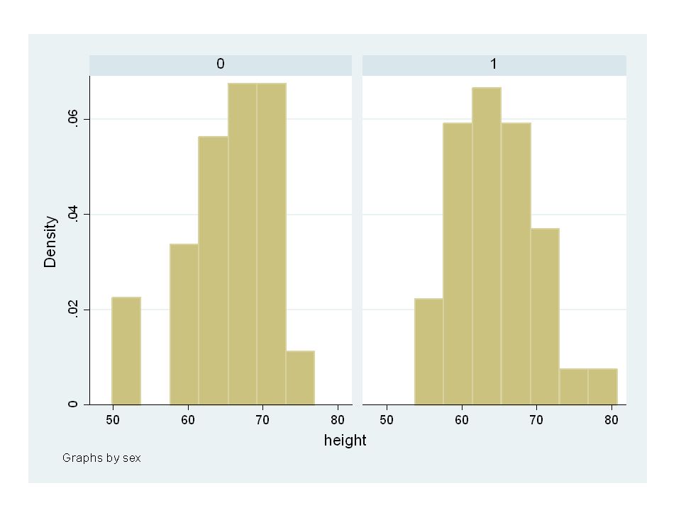
Creating Histograms Stata command: hist Example: Histogram of height, by sex hist height, by(sex)
")
11
Creating Histograms Stata command: hist Attach value labels to variable(s) of interest Use formatting options Example revisited: Histogram of height, by sex hist height, by(sex, title(“Distribution of height by sex”) note(“”)) xtitle(“height(in)”) scheme(s1mono)
 of interest Use formatting options Example revisited: Histogram of height, by sex hist height, by(sex, title( Distribution of height by sex ) note( )) xtitle( height(in) ) scheme(s1mono)")
13
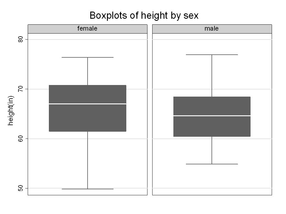
Creating Box Plots Stata command: graph box Example: Box plot of height, by sex graph box height, by(sex, title(Boxplots of height by sex) note(“”)) ytitle(height(in)) scheme(s1mono)
 note( )) ytitle(height(in)) scheme(s1mono)")
15
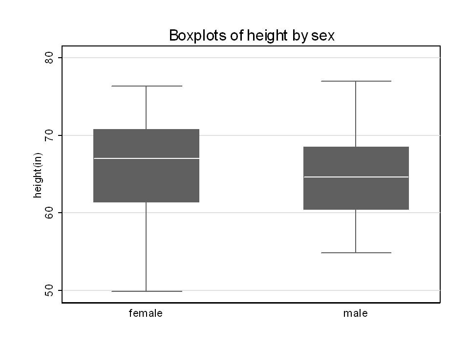
Creating Box Plots Stata command: graph box Now using over option Example: Box plot of height, by sex graph box height, over(sex) title(“Boxplots of height by sex”) ytitle(“height(in)”) scheme(s1mono)
 title( Boxplots of height by sex ) ytitle( height(in) ) scheme(s1mono)")
17
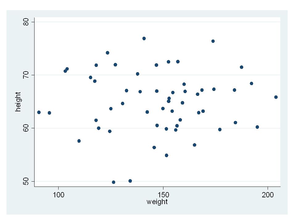
Creating Scatter Plots Stata command: scatter Example: Scatter plot of height and weight scatter height weight

19
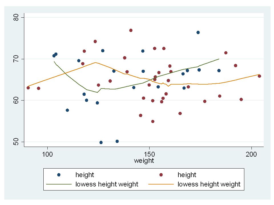
Creating Scatter Plots Stata command: scatter Example: Scatter plot of height and weight by sex, with lowess smoothing twoway (scatter height weight if sex==0) /// (scatter height weight if sex==1) /// (lowess height weight if sex==0) /// (lowess height weight if sex==1)
 /// (scatter height weight if sex==1) /// (lowess height weight if sex==0) /// (lowess height weight if sex==1)")
21
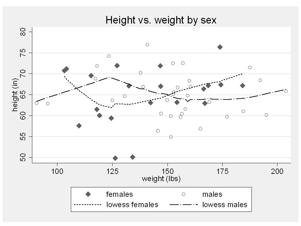
Creating Scatter Plots Stata command: scatter Use formatting options Example revisited: Scatter plot of height and weight by sex, with lowess smoothing twoway(scatter height weight if sex==0,ms(D)) (scatter height weight if sex==1, ms(Oh)) (lowess height weight if sex==0) (lowess height weight if sex==1),scheme(s2mono) legend(col(2)order(1 “females” 2 “males” 3 “lowess females” 4 “lowess males”)) xtitle(weight(lbs)) ytitle(height(in)) title(Height vs. weight by sex) xlab(100(25)200) ylab(50(5)80)
 xlab(100(25)200) ylab(50(5)80).")
23
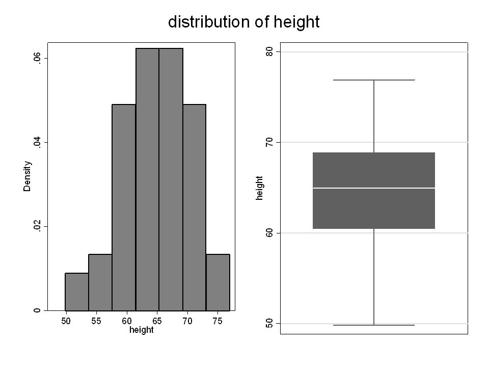
Combining Graphs Stata command: graph combine Example: Histogram and box plot of height hist height, scheme(s1mono) name(hist) graph box height, scheme(s1mono) name(box) graph combine hist box, scheme(s1mono) title(distribution of height)
 name(hist) graph box height, scheme(s1mono) name(box) graph combine hist box, scheme(s1mono) title(distribution of height)")
Similar presentations


.>")


 Discussion Section Week 4 Sandrine Moutou Medical Biometry I.>")

, or Quetelet index, is a measure for human body shape based on an individual's weight and height.>")


 The breaking strength in pounds of force is being studied for two metal alloys, labeled S and T, and for different temperatures.>")


 This is the most commonly used index of over or underweight Body Mass Index = body weight ( Height) squared ClassificationBMI.>")