1. 1 ECON 240A Power 5

2. 2 Last Week b Probability b Discrete Binomial Probability Distribution

3. 3 The Normal Distribution

4. 4 Outline b The normal distribution as an approximation to the binomial b The standardized normal variable, z b sample means

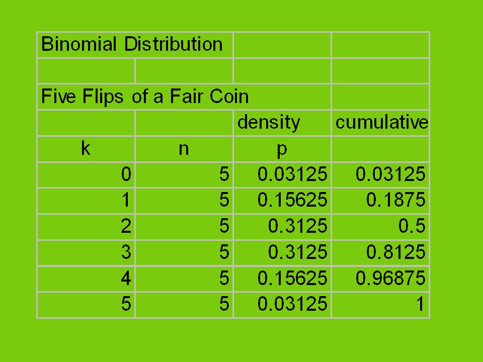
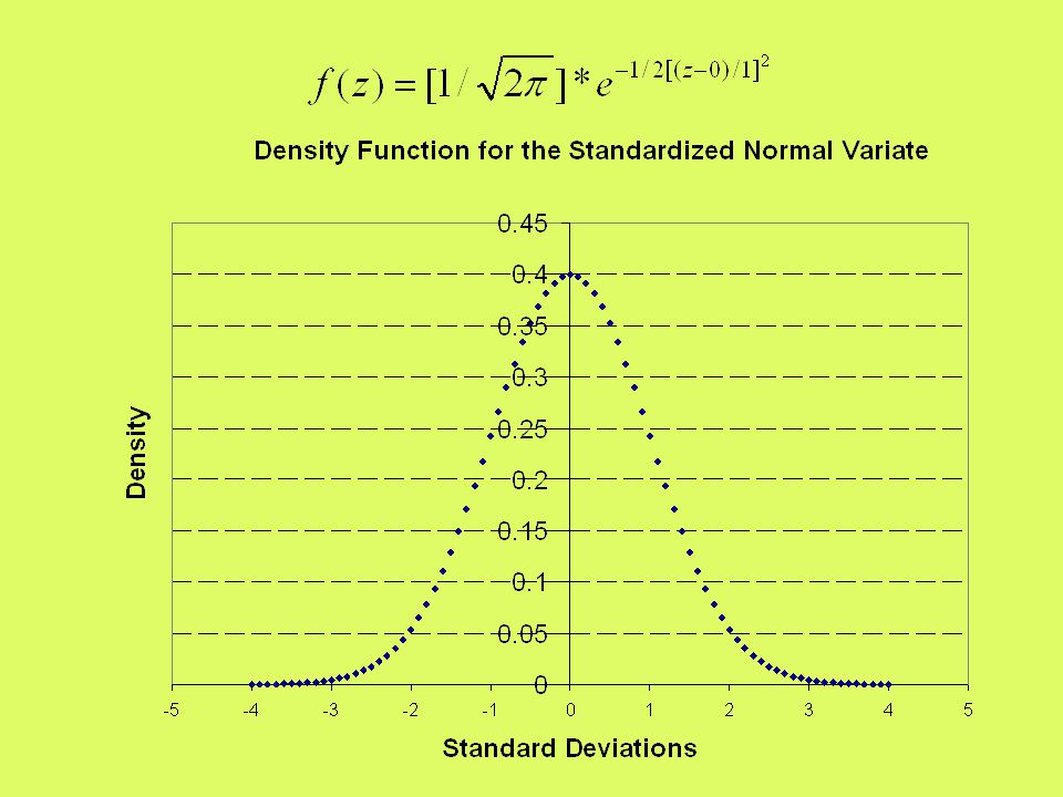
6. 6 Probability Density Function

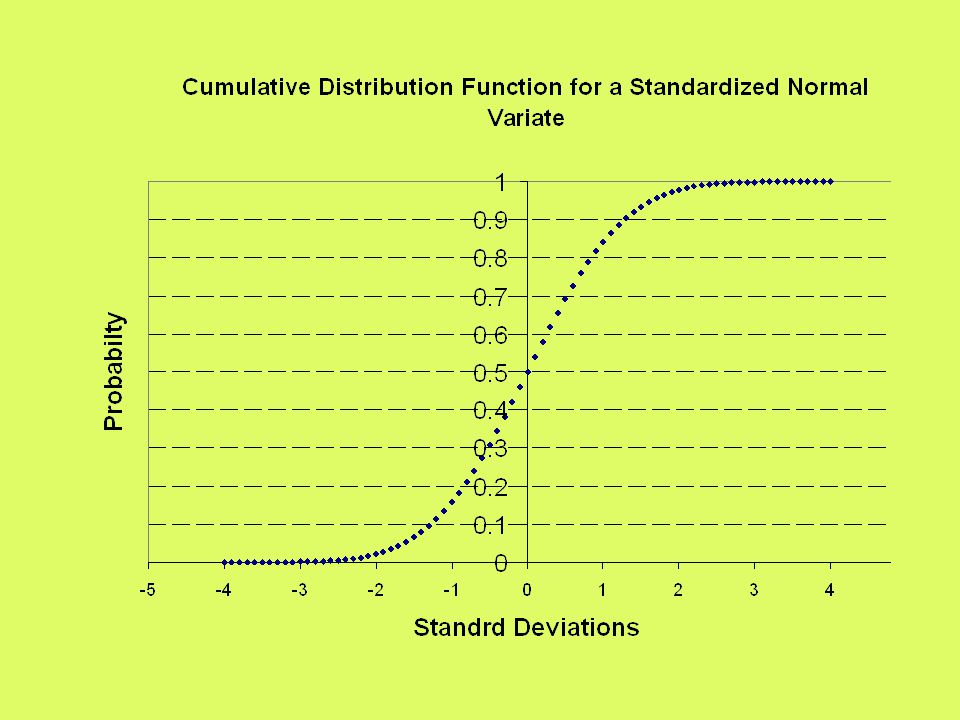
7. 7 Cumulative Distribution Function

8. 8 b The probability of getting two or less heads in five flips is 0.5 can use the cumulative distribution functioncan use the cumulative distribution function can use the probability density function and add the probabilities for 0, 1, and 2 headscan use the probability density function and add the probabilities for 0, 1, and 2 heads b the probability of getting two heads or three heads is can add the probabilities for 2 heads and three heads from the probability density functioncan add the probabilities for 2 heads and three heads from the probability density function

9. 9 Cumulative Distribution Function

11. 11 Cumulative Distribution Function b the probability of getting two heads or three heads is: can add the probabilities for 2 heads and three heads from the probability density functioncan add the probabilities for 2 heads and three heads from the probability density function can use the probability of getting up to 3 heads, P(3 or less heads) from the cumulative distribution function (CDF) and subtract the probability of getting up to one head P(1 or less heads]can use the probability of getting up to 3 heads, P(3 or less heads) from the cumulative distribution function (CDF) and subtract the probability of getting up to one head P(1 or less heads]

12. 12 Probability Density Function

15. 15 Cumulative Distribution Function

16. 16 For the Binomial Distribution b Can use a computer as we did in Lab Two b Can use Tables for the cumulative distribution function of the binomial such as Table 1 in the text in Appendix B, p. B-1 need a table for each p and n.need a table for each p and n.

17. 17

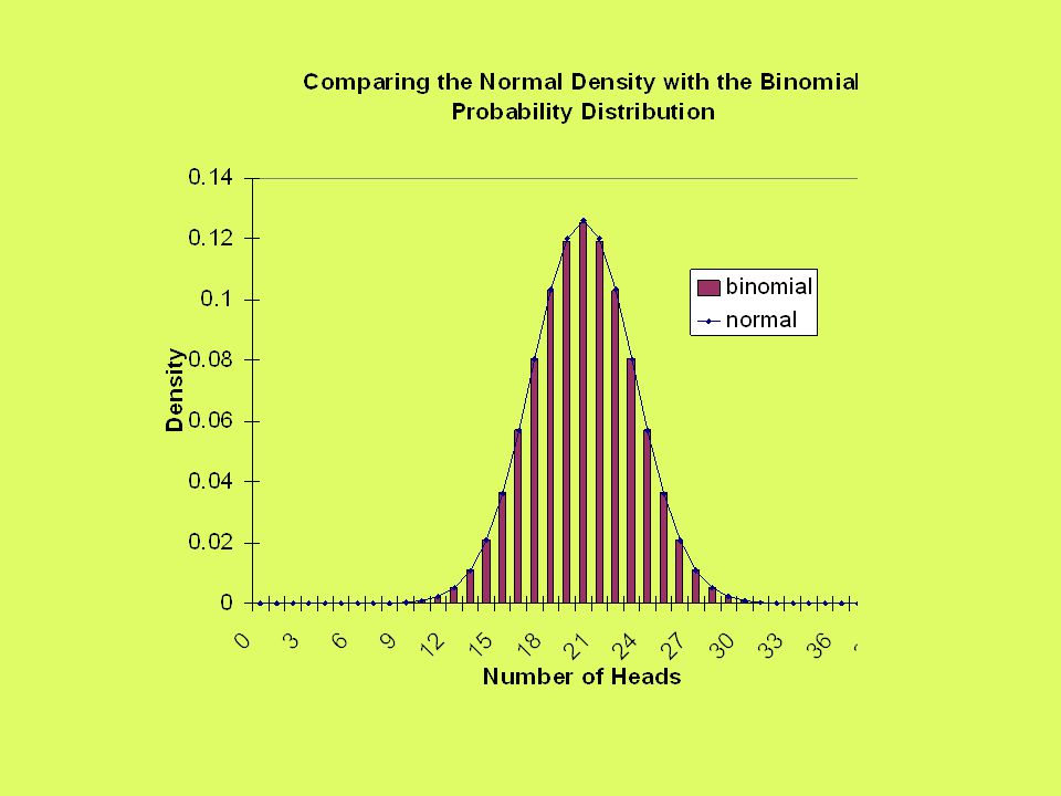
18. 18 Normal Approximation to the binomial b Fortunately, for large samples, we can approximate the binomial with the normal distribution, as we saw in Lab Two

19. Binomial Probability Density Function

20. Binomial Cumulative Distribution Function

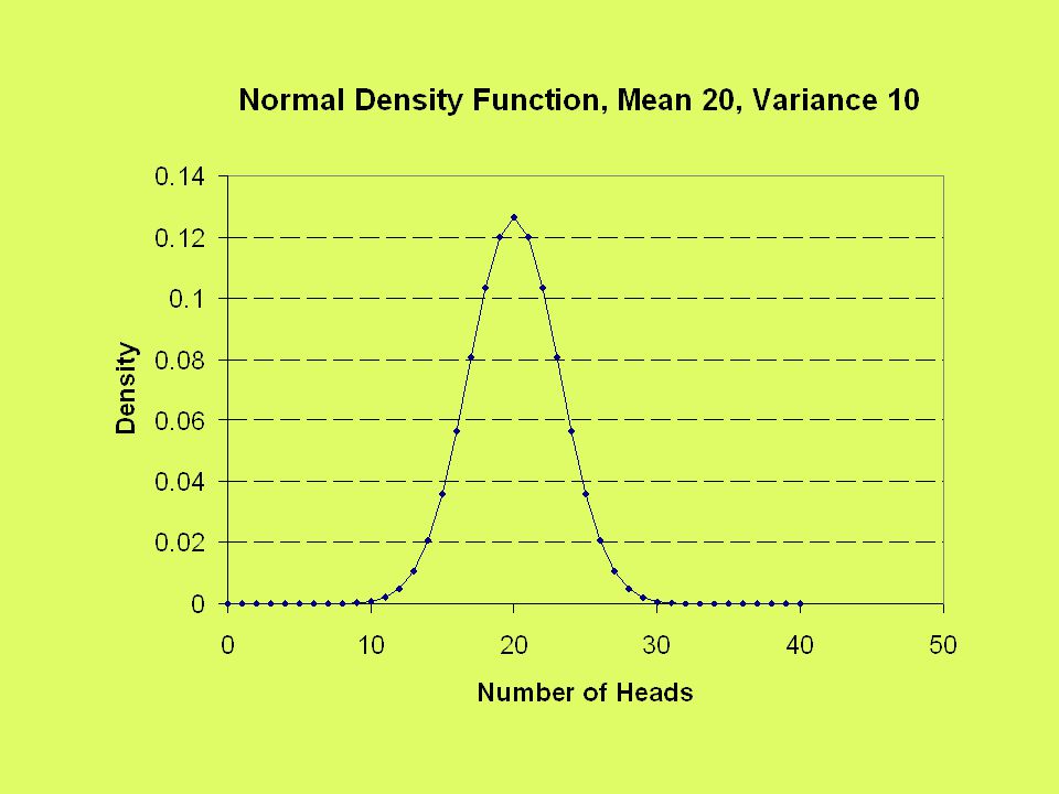
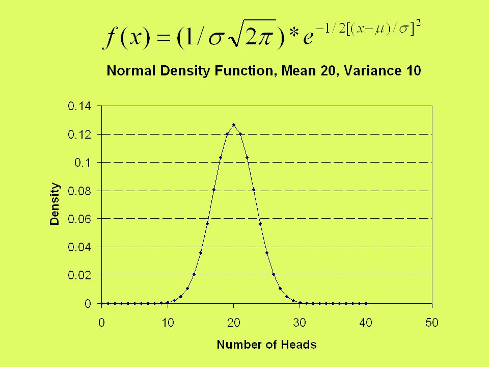
21. 21 The Normal Distribution b What would the normal density function look like if it had the same expected value and the same variance as this binomial distribution from Power 4, E(h) = n*p =40*1/2=20from Power 4, E(h) = n*p =40*1/2=20 from Power 4, VAR[h] = n*p*(1-p) = 40*1/2*1/2 =10from Power 4, VAR[h] = n*p*(1-p) = 40*1/2*1/2 =10

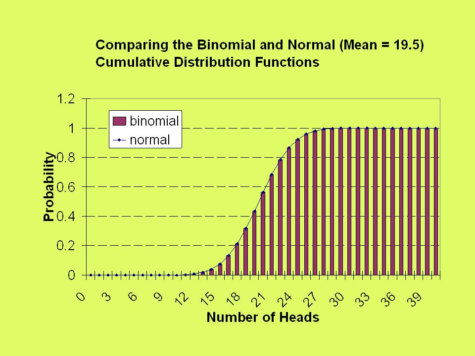
26. Normal Approximation to the Binomial: De Moivre This is the probability that the number of heads will fall in the interval a through b, as determined by the normal cumulative distribution function, using a mean of n*p, and a standard deviation equal to the square root of n*p*(1-p), i.e. the square root of the variance of the binomial distribution. The parameter 1/2 is a continuity correction since we are approximating a discrete function with a continuous one, and was the motivation of using mean 19.5 instead of mean 20 in the previous slide. Visually, this seemed to be a better approximation than using a mean of 20.

27. 27 Guidelines for using the normal approximation b n*p>=5 b n*(1-p)>=5

28. 28 The Standardized Normal Variate b Z~N(0, 10] b E[z} = 0 b VAR[Z] = 1

31. Normal Variate x –E(z) = 0 –VAR(z) = 1

33. b

34. b

35. 35 For the Normal Distribution b Can use a computer as we did in Lab Two b Can use Tables for the cumulative distribution function of the normal such as Table 3 in the text in Appendix B, p. B-8 need only one table for the standardized normal variate Z.need only one table for the standardized normal variate Z.

36. 36

37. 37 Sample Means

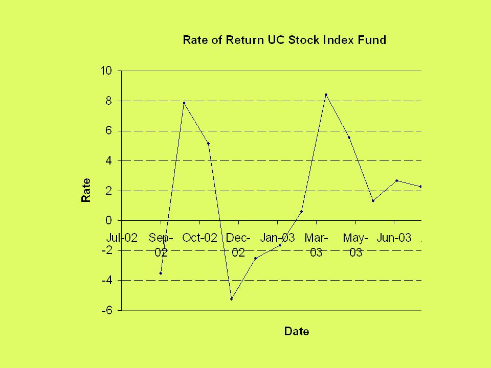
38. 38 Sample Mean Example b Rate of return on UC Stock Index Fund b return equals capital gains or losses plus dividends b monthly rate of return equals price this month minus price last month, plus dividends, all divided by the price last month b r(t) ={ p(t) -p(t-1) + d(t)}/p(t-1)

39. 39 Rate of Return UC Stock Index Fund, http://atyourservice.ucop.edu/

40. 40 Table Cont.

42. 42 Data Considerations b Time series data for monthly rate of return b since we are using the fractional change in price (ignoring dividends) times 100 to convert to %, the use of changes approximately makes the observations independent of one another b in contrast, if we used price instead of price changes, the observations would be correlated, not independent

43. Cont. b b assume a fixed target, i.e. the central tendency of the rate is fixed, not time varying b b Assume the rate has some distribution, f, other than normal: r i = b b sample mean:

44. 1.74

45. 45 What are the properties of this sample mean?

46. Note: Expected value of a constant, c, times a random variable, x(i), where i indexes the observation Note: Variance of a constant times a random variable VAR[c*x] = E{cx - E[c*x]} 2 = E{c*[x-Ex]} 2 = E{c 2 [x -Ex] 2 } = c 2 *E[x-Ex] 2 = c 2 *VARx

47. Properties of b b Expected value: b b Variance

48. 48 Central Limit Theorem b As the sample size grows, no matter what the distribution, f, of the rate of return, r, the distribution of the sample mean approaches normality

49. b b An interval for the sample mean

50. 50 The rate of return, r i The rate of return, r i, could be distributed as uniform f[r(i)] r(i)

51. 51 And yet for a large sample, the sample mean will be distributed as normal a b

52. 52 Bottom Line b We can use the normal distribution to calculate probability statements about sample means

53. b b An interval for the sample mean calculate choose infer ?, Assume we know, or use sample standard deviation, s

54. Sample Standard Deviation b b If we use the sample standard deviation, s, then for small samples, approximately less then 100 observations, we use Student’s t distribution instead of the normal

55. 55 Text p.253 Normal compared to t t-distribution t distribution as smple size grows

56. 56 Appendix B Table 4 p. B-9