Download presentation
Presentation is loading. Please wait.

1
The Empirical Mode Decomposition Method Sifting

2
Goal of Data Analysis To define time scale or frequency. To define energy density. To define joint frequency-energy distribution as a function of time. To do this, we need a AM-FM decomposition of the signal. X(t) = A(t) cosθ(t), where A(t) defines local energy and θ(t) defines the local frequency.
 = A(t) cosθ(t), where A(t) defines local energy and θ(t) defines the local frequency..")
3
Need for Decomposition Hilbert Transform (and all other IF computation methods) only offers meaningful Instantaneous Frequency for IMFs. For complicate data, there should be more than one independent component at any given time. The decomposition should be adaptive in order to study data from nonstationary and nonlinear processes. Frequency space operations are difficult to track temporal changes.

4
Why Hilbert Transform not enough? Even though mathematicians told us that the Hilbert transform exists for all functions of Lp-class.

5
Problems on Envelope A seemingly simple proposition but it is not so easy.

6
Two examples

7
Data set 1

8
Data X1

9
Data X1 Hilbert Transform

10
Data X1 Envelopes

11
Observations None of the two envelopes seem to make sense: The Hilbert transformed amplitude oscillates too much. The line connecting the local maximum is almost the tracing of the data. It turns out that, though Hilbert transform exists, the simple Hilbert transform does not make sense. For envelopes, the necessary condition for Hilbert transformed amplitude to make sense is for IMF.

12
Data X1 IMF

13
Data x1 IMF1

14
Data x2 IMF2

15
Observations For each IMF, the envelope will make sense. For complicate data, we have to decompose it before attempting envelope construction. To be able to determine the envelope is equivalent to AM & FM decomposition.

16
Data set 2

17
Data X2

18
Data X2 Hilbert Transform

19
Data X2 Envelopes

20
Observations Even for this well behaved function, the amplitude from Hilbert transform does not serve as an envelope well. One of the reasons is that the function has two spectrum lines. Complications for more complex functions are many. The empirical envelope seems reasonable.

21
Empirical Mode Decomposition Mathematically, there are infinite number of ways to decompose a functions into a complete set of components. The ones that give us more physical insight are more significant. In general, the few the number of representing components, the higher the information content. The adaptive method will represent the characteristics of the signal better. EMD is an adaptive method that can generate infinite many sets of IMF components to represent the original data.

22
Empirical Mode Decomposition: Methodology : Test Data

23
Empirical Mode Decomposition: Methodology : data and m1

24
Empirical Mode Decomposition: Methodology : data & h1

25
Empirical Mode Decomposition: Methodology : h1 & m2

26
Empirical Mode Decomposition: Methodology : h2 & m3

27
Empirical Mode Decomposition: Methodology : h3 & m4

28
Empirical Mode Decomposition: Methodology : h2 & h3

29
Empirical Mode Decomposition: Methodology : h4 & m5

30
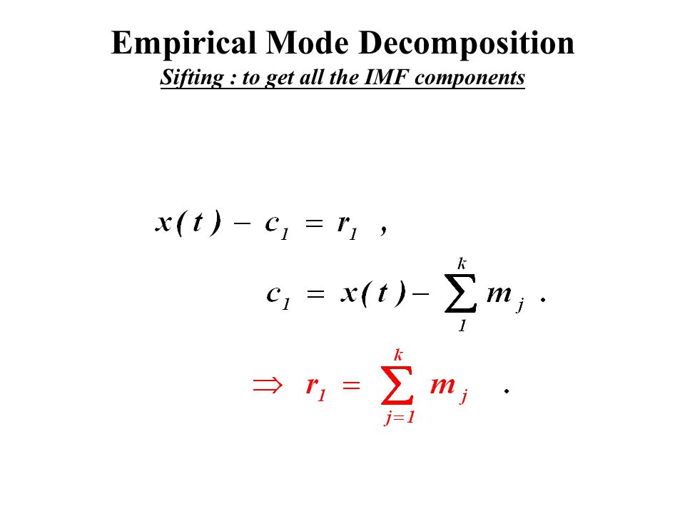
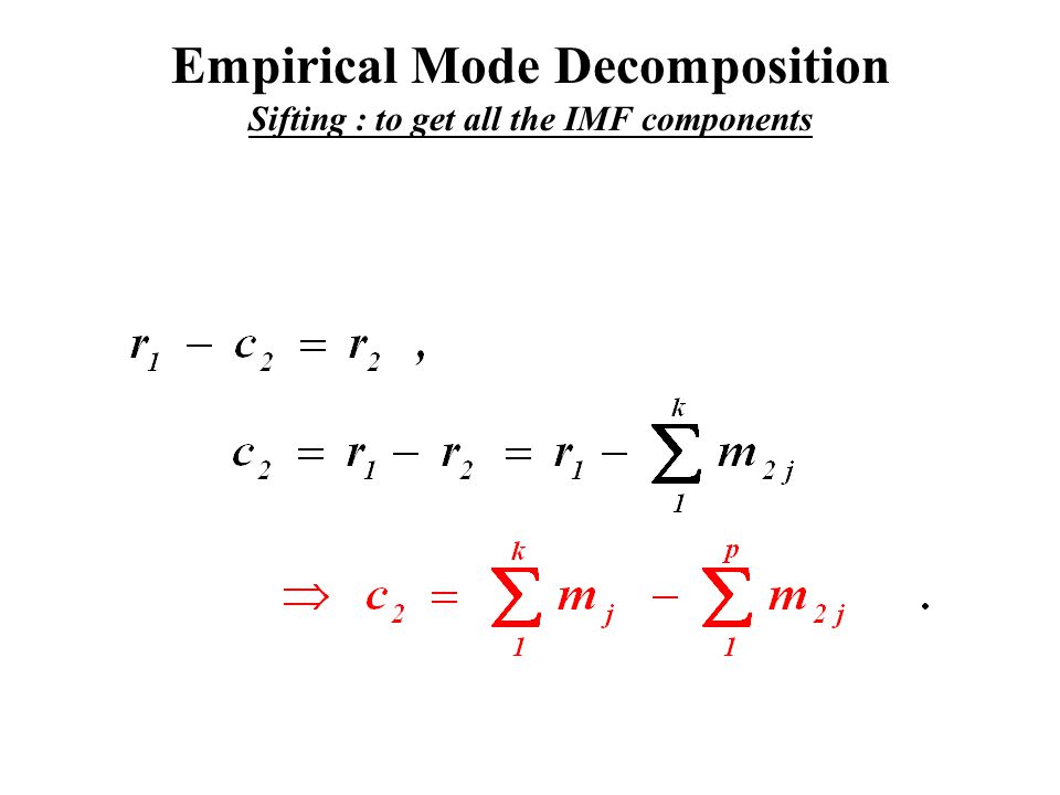
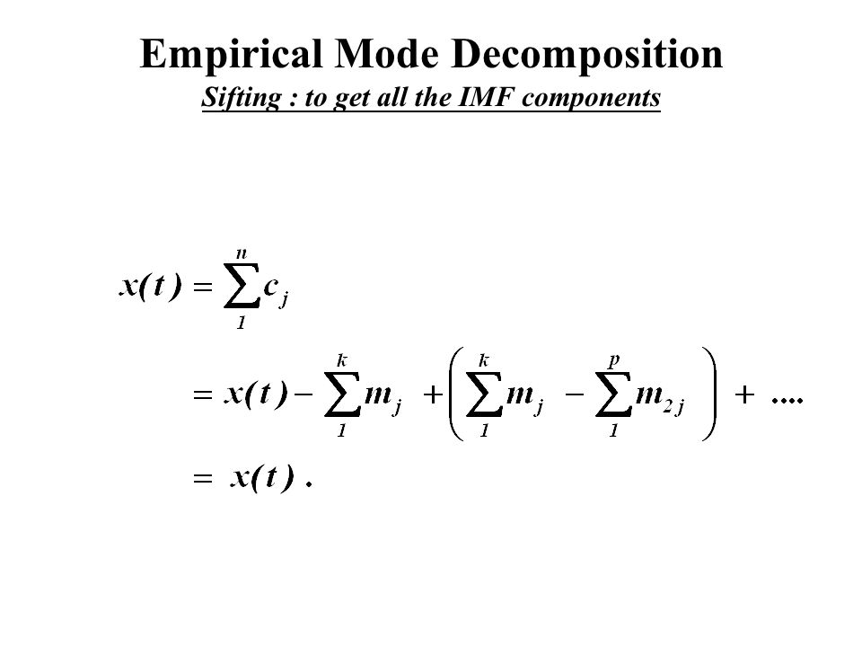
Empirical Mode Decomposition Sifting : to get one IMF component

32
Empirical Mode Decomposition: Methodology : IMF c1

33
Definition of the Intrinsic Mode Function

34
Empirical Mode Decomposition Sifting : to get all the IMF components

38
Empirical Mode Decomposition: Methodology : data & r1

39
Empirical Mode Decomposition: Methodology : data, h1 & r1

40
Empirical Mode Decomposition: Methodology : IMFs

41
Definition of Instantaneous Frequency

42
Definitions of Frequency

43
The Effects of Sifting The first effect of sifting is to eliminate the riding waves : to make the number of extrema equals to that of zero-crossing. The second effect of sifting is to make the envelopes symmetric. The consequence is to make the amplitudes of the oscillations more even.

44
Singularity points for Instantaneous Frequency

45
Critical Parameters for EMD The maximum number of sifting allowed to extract an IMF, N. The criterion for accepting a sifting component as an IMF, the Stoppage criterion S. Therefore, the nomenclature for the IMF are CE(N, S) : for extrema sifting CC(N, S) : for curvature sifting
 : for extrema sifting CC(N, S) : for curvature sifting.")
46
The Stoppage Criteria : S and SD A. The S number : S is defined as the consecutive number of siftings, in which the numbers of zero- crossing and extrema are the same for these S siftings. B. If the mean is smaller than a pre-assigned value. C. SD is small than a pre-set value, where

47
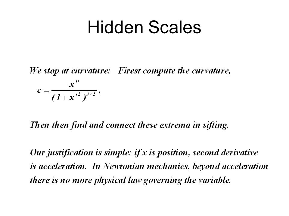
Curvature Sifting Hidden Scales

48
Empirical Mode Decomposition: Methodology : Test Data

49
Hidden Scales

51
Observations If we decide to use curvature, we have to be careful for what we ask for. For example, the Duffing pendulum would produce more than one components. Therefore, curvature sifting is used sparsely. It is useful in the first couple of components to get rid of noises.

52
Intermittence Test To alleviate the Mode Mixing

53
Sifting with Intermittence Test To avoid mode mixing, we have to institute a special criterion to separate oscillation of different time scales into different IMF components. The criteria is to select time scale so that oscillations with time scale shorter than this pre- selected criterion is not included in the IMF.

54
Intermittence Sifting : Data

55
Intermittence Sifting : IMF

56
Intermittence Sifting : Hilbert Spectra

57
Intermittence Sifting : Hilbert Spectra (Low)
")
58
Intermittence Sifting : Marginal Spectra

59
Intermittence Sifting : Marginal spectra (Low)
")
60
Intermittence Sifting : Marginal spectra (High)
")
61
Critical Parameters for Sifting Because of the inclusion of intermittence test there will be one set of intermittence criteria. Therefore, the Nomenclature for IMF here are CEI(N,S: n1, n2, …) CCI(N, S: n1, n2, …) with n1, n2 as the intermittence test criteria.
 CCI(N, S: n1, n2, …) with n1, n2 as the intermittence test criteria..")
62
The mathematical Requirements for Basis The traditional Views

63
IMF as Adaptive Basis According to the established mathematical paradigm, we should check the following properties of the basis: Convergence completeness orthogonality Uniqueness

64
Convergence

65
Convergence Problem Given an arbitrary number, ε, there always exists a large finite number N, such that Nth envelope mean, m N, satisfies | m N | ≤ε:

66
Convergence Problem Given an arbitrary number, ε, there always exists a large finite number N, such that N- th sifting satisfies

67
Convergence There is another convergence problem: we have only finite number of components. Complete proof for convergence is underway. We can prove the convergence under simplified condition of linear segment fitting for sifting. Empirically, we found all cases converge in finite steps. The finite component, n, is less than or equal to log 2 N, with N as the total number of data points.

68
Convergence The necessary condition for convergence is that the mean line should have less extrema than the original data. This might not be true if we use the middle points and a single spline; the procedure might not converge.

69
Completeness

70
Completeness is given by the algebraic equation Therefore, the sum of IMF can be as close to the original data as required. Completeness is given.

71
Orthogonality

72
Definition: Two vectors x and y are orthogonal if their inner product is zero. x ∙y = (x 1 y 1 + x 2 y 2 + x 3 y 3 + … ) = 0.
 = 0..")
73
The need for an orthogonality check Orthogonal is required for:

74
Orthogonality Orthogonality is a requirement for any linear decomposition. For a nonlinear decomposition, as EMD, the orthogonality should not be a requirement, for nonlinear waves of different scale could share the same harmonics. Fortunately, the EMD is basically a Reynolds type decomposition, U = + u’, orthogonality is always approximately satisfied to the degree of nonlinearity. Orthogonality Index should be checked for each cases as a goodness of decomposition confirmation.

75
Orthogonality Index

76
Length Of Day Data

77
LOD : IMF

78
Orthogonality Check Pair-wise % 0.0003 0.0001 0.0215 0.0117 0.0022 0.0031 0.0026 0.0083 0.0042 0.0369 0.0400 Overall % 0.0452

79
Uniqueness

80
EMD, with different critical parameters, can generate infinite sets of IMFs. The result is unique only with respect to the critical parameters and sifting method selected; therefore, all results should be properly named according to the nomenclature scheme proposed above. The present sifting is based on cubic spline. Different spline fitting in the sifting procedure will generate different results. The ensemble of IMF sets offers a Confidence Limit as function of time and frequency.

81
Some Tricks in Sifting

82
Sometimes straightforward application of sifting will not generate good results. Invoking intermittence criteria is an alternative to get physically meaningful IMF components. By adding low level noise can improve the sifting. By using curvature may also help.

83
An Example Adding Noise of small amplitude only, A prelude to the true Ensemble EMD

84
Data: 2 Coincided Waves

85
IMF from Data of 2 Coincided Waves

86
Data: 2 Coincided Waves + Noise The Amplitude of the noise is 1/1000

87
IMF form Data 2 Coincided Waves + Noise

88
IMF c1 and Component2 : 2 Coincided Waves

89
IMF c2+c3 and Component1 : 2 Coincided Waves

90
A Flow Chart Data IMF sifting With Intermittence Hilbert Spectrum IF Marginal Spectrum OI CL Ensemble EMD

Similar presentations