1. On the Trend, Detrend and the Variability of Nonlinear and Nonstationary Time Series A new application of HHT

2. Satellite Altimeter Data : Greenland

3. Two Sets of Data

4. The State-of-the-Arts “ One economist’s trend is another economist’s cycle” Engle, R. F. and Granger, C. W. J. 1991 Long-run Economic Relationships. Cambridge University Press. Simple trend – straight line Stochastic trend – straight line for each quarter

5. Philosophical Problem 名不正則言不順 言不順則事不成 —— 孔夫子

6. On Definition Without a proper definition, logic discourse would be impossible. Without logic discourse, nothing can be accomplished. Confucius

7. Definition of the Trend Within the given data span, the trend is an intrinsically fitted monotonic function, or a function in which there can be at most one extremum. The trend should be determined by the same mechanisms that generate the data; it should be an intrinsic and local property. Being intrinsic, the method for defining the trend has to be adaptive. The results should be intrinsic (objective); all traditional trend determination methods give extrinsic (subjective) results. Being local, it has to associate with a local length scale, and be valid only within that length span as a part of a full wave cycle.

8. Definition of Detrend and Variability Within the given data span, detrend is an operation to remove the trend. Within the given data span, the Variability is the residue of the data after the removal of the trend. As the trend should be intrinsic and local properties of the data; Detrend and Variability are also local properties. All traditional trend determination methods are extrinsic and/or subjective.

9. The Need for HHT HHT is an adaptive (local, intrinsic, and objective) method to find the intrinsic local properties of the given data set, therefore, it is ideal for defining the trend and variability.

10. History of HHT 1998: The Empirical Mode Decomposition Method and the Hilbert Spectrum for Non-stationary Time Series Analysis, Proc. Roy. Soc. London, A454, 903-995. The invention of the basic method of EMD, and Hilbert transform for determining the Instantaneous Frequency and energy. 1999: A New View of Nonlinear Water Waves – The Hilbert Spectrum, Ann. Rev. Fluid Mech. 31, 417-457. Introduction of the intermittence in EMD. 2003: A confidence Limit for the Empirical mode decomposition and the Hilbert spectral analysis, Proc. of Roy. Soc. London, A459, 2317-2345. Establishment of a confidence limit without the ergodic assumption. 2004: A Study of the Characteristics of White Noise Using the Empirical Mode Decomposition Method, Proc. Roy. Soc. London, (in press) Defined statistical significance and predictability of IMFs. 2004: On the Instantaneous Frequency, Proc. Roy. Soc. London, (Under review) Removal of the limitations posted by Bedrosian and Nuttall theorems for instantaneous Frequency computations.

11. Two Sets of Data

12. Global Temperature Anomaly Annual Data from 1856 to 2003

13. Global Temperature Anomaly 1856 to 2003

14. IMF Mean of 10 Sifts : CC(1000, I)

15. Mean IMF

16. STD IMF

17. Statistical Significance Test

18. Data and Trend C6

19. Data and Overall Trends : EMD and Linear

20. Rate of Change Overall Trends : EMD and Linear

21. Variability with Respect to Overall trend

22. Data and Trend C5:6

23. Data and Trends: C5:6

24. Rate of Change Trend C5:6

25. Trend Period C5

26. Variability with Respect to 65-Year trend

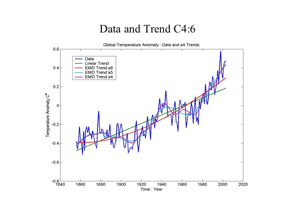
27. Data and Trend C4:6

29. Rate of Change Trend C4:6

30. Trend Period C4

31. Variability with Respect to 20-Year trend

32. Data and Trend C3:6

33. Trend Period C3

34. Histogram of Trend Period C3

35. Variability with Respect to 10-Year trend

36. Hilbert Spectrum Global Temperature Anomaly

37. Marginal Hilbert Spectrum

38. Morlet Wavelet Spectrum

39. Hilbert and Morlet Wavelet Spectra

40. Financial Data : NasDaqSC October 11, 1984 – December 29, 2000 October 12, 2004

41. NasDaq Data

42. NasDaq IMF

43. NasDaq IMF Reconstruction : A

44. NasDaq IMF Reconstruction : B

45. NasDaq Various Overall Trends

46. NasDaq various Overall Detrends Mean : L = 0 Exp = 73.1187 EMD = 0.3588 STD : L = 559.09 Exp = 426.66 EMD = 238.10

47. NasDaq Trend IMF (C8-C9)

48. NasDaq Local Period for Trend IMF (C8-C9) mean = 796.6

49. NasDaq Trend IMF (C7-C9)

50. NasDaq Local Period for Trend IMF (C7-C9) Mean = 425.7

51. NasDaq Trend IMF (C6-C9)

52. NasDaq Local Period for Trend IMF (C6-C9) Mean = 196.5

53. NasDaq Traditional Moving Mean Trends: Details

54. NasDaq Trends: Moving Mean and EMD : Details

55. NasDaq Period of EMD Trend (C4) Mean = 35.56

56. NasDaq Distribution of Period for EMD Trend (C4)

57. NasDaq Detrended Data (C4-C9)

58. NasDaq Detrended Data (C4-C9) : Details

59. NasDaq Histogram Detrended Data (C1-C3)

60. Various Definitions of Variability Variability defined by percentage Gain is the absolute value of the Gain. Variability defined by daily high-low is the percentage of absolute value of High-Low. Variability defined by Empirical Mode Decomposition is the percentage of the absolute value of the sum from selected IMFs. Financial data do not look like ARIMA.

61. NasDaq Variability defined by EMD : C1

62. NasDaq Variability defined by Gain

63. NasDaq Variability defined by Daily High-Low

64. NasDaq Period of Variability defined by EMD : C1 Mean = 8.38

65. NasDaq Histogram Period of EMD Variability : C1

66. NASDAQ Price gradient vs. Gain Variability

67. NASDAQ Price gradient vs. High-Low Variability

68. NASDAQ Price gradient vs. EMD Variability

69. Relationship between Variability: Gain vs. EMD

70. Relationship between Variability: Gain vs. High- Low

71. Relationship between Variability: EMD vs. High- Low

72. Statistical Significance Test for IMF

73. Methodology Based on observations from Monte Carlo numerical experiments on 1 million white noise data points. All IMF generated by 10 siftings. Fourier spectra based on 200 realizations of 4,000 data points sections. Probability density based on 50,000 data points data sections.

74. IMF Period Statistics IMF 123456789 number of peaks 34704216817683456416322087710471529026581348 Mean period2.8815.94611.9824.0247.9095.50189.0376.2741.8 period in year0.2400.4960.9982.0003.9927.95815.7531.3561.75

75. Fourier Spectra of IMFs

76. Empirical Observations : I Normalized spectral area is constant

77. Empirical Observations : II Computation of mean period

78. Empirical Observations : III The product of the mean energy and period is constant

79. Monte Carlo Result : IMF Energy vs. Period

80. Empirical Observation: Histograms IMFs By Central Limit theory IMF should be normally distributed.

81. Histograms : IMF Energy Density By Central Limit theory, IMF should be normally distributed; therefore, its energy should be Chi-squared distributed.

82. Chi-Squared Energy Density Distributions By Central Limit theory, IMF should be normally distributed; therefore, its energy should be Chi-squared distributed.

83. Formula of Confidence Limit for IMF Distributions Introduce new variable y: Then,

84. Confidence Limit for IMF Distributions

85. Data and IMFs SOI

86. Statistical Significance for SOI IMFs 1 mon1 yr10 yr100 yr IMF 4, 5, 6 and 7 are 99% statistical significance signals.

87. Summary Not all IMF have the same statistical significance. Based on the white noise study, we have established a method to determine the statistical significant components. References: Wu, Zhaohua and N. E. Huang, 2003: A Study of the Characteristics of White Noise Using the Empirical Mode Decomposition Method, Proceedings of the Royal Society of London (in press) Flandrin, P., G. Rilling, and P. Gonçalvès, 2003: Empirical Mode Decomposition as a Filterbank, IEEE Signal Processing, (in press).

88. Statistical Significance Test Only the statistical Significant IMF components are signal above noise; therefore, they might be predictable.

89. Statistical Significance Test : Gain

90. Statistical Significance Test : High-Low

91. Statistical Significance Test : EMD

92. Statistical Significance Test : All Variability Definitions

93. The Sum of all the Statistical Significance IMFs

94. Relationship among Trends: Gain vs. EMD

95. Relationship among Trends: Gain vs. High-Low

96. Relationship among Trends: EMD vs. High-Low

97. Summary A working definition for the trend is established; it is a function of the local time scale. Need adaptive method to analysis nonstationary and nonlinear data for trend and variability Various definitions for variability should be compared in details to determine their significance.