1. Geol 600 Notable Historical Earthquakes Finite fault rupture propagation http://www- rohan.sdsu.edu/~kbolsen/geol600_nhe_source_inversion.ppt

2. 9 Force Couples M ij (the moment tensor), 6 different (M ij =M ji ). |M|=fd M 11 M 12 M 13 Good approximation for distant M= M 21 M 22 M 23 earthquakes due to a point source M 31 M 32 M 33 Larger earthquakes can be modeled as sum of point sources

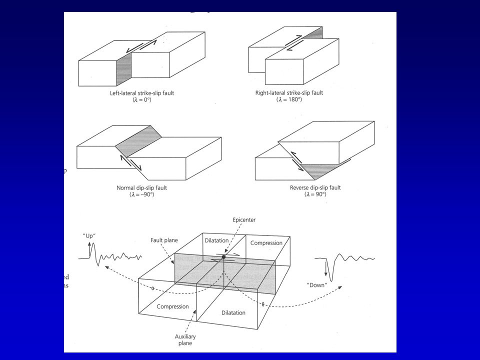
3.  Description of earthquakes using moment tensors: Parameters: strike , dip , rake Right-lateral =180 o, left-lateral =0 o, =90 reverse, =-90 normal faulting Strike, dip, rake, slip define the focal mechanism

4.  Description of earthquakes using moment tensors: M 11 = -M 0 (sin  cos sin2  s + sin2  sin sin 2  s ), M 12 = M 0 (sin  cos cos2  s + 0.5 sin2  sin sin2  s ), M 13 = -M 0 (cos  cos cos  s + cos2  sin sin  s ), M 22 = M 0 (sin  cos sin2  s - sin2  sin cos 2  s ), M 23 = -M 0 (cos  cos sin  s - cos2  sin cos  s ), M 33 = M 0 sin2  sin 

5. P-waves S-waves

8. Finite-size Fault Plane Divide into ‘sub-faults’ ‘sub-faults’ x x x x

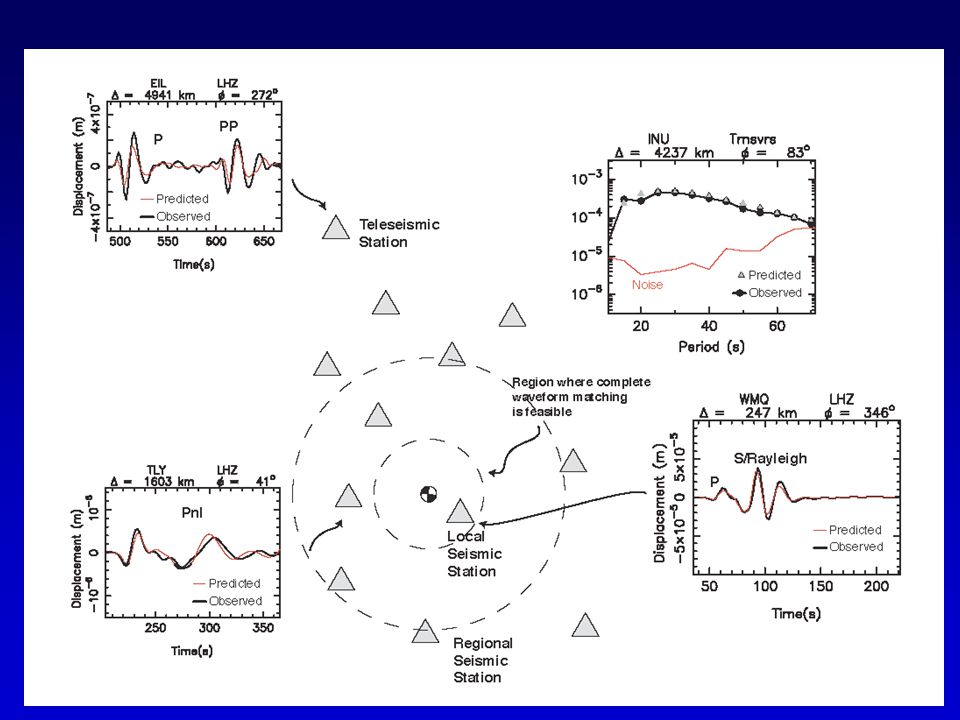
9. Define rupture parameters (distributions of slip, rake, rupture speed, source-time function, stress, friction, etc) wave-propagation code Compute synthetic seismograms at receiver locations Compare synthetic to observed seismograms Synthetics fit data? Yes no

10. Kinematic source inversion: Solves for slip history on the fault Dynamic source inversion: Solves for stress and friction on the fault

11. Kinematic Source Inversion

12. Landers: Classic Vertical Strike-Slip Event

14. Test case: 1992 M 7.3 Landers Well-recorded event

15. Slip-weakening Rupture Model

16. Dynamic Rupture From Trial-and-Error Finite-Difference Modeling

17. How is rupture propagation affected by realistic variation of dynamic parameters? Let’s look at changes in the stress drop…

18. Inverted (Trial-and- Error) Dynamic Radiation Versus Data

19. Stress Field (a)

20. Stress Field (b)

21. Stress Field (c)

22. 1994 M6.7 Northridge

24. 2004 M6.0 Parkfield

26. 1999 M7.4 Izmit

27. SOURCE TIME FUNCTION DURATION ALSO VARIES WITH STATION AZIMUTH FROM FAULT. THIS DIRECTIVITY CAN CONSTRAIN WHICH NODAL PLANE IS THE FAULT PLANE For earthquake, V/V R ~1.2 for shear waves and 2.2 for P waves. Maximum duration is 180° from the rupture direction, and the minimum is in the rupture direction. Analogous effect: thunder generated by sudden heating of air along a lightning channel in the atmosphere. Here V/V R ~0, so observers perpendicular to the channel hear a brief, loud, thunder clap, whereas observers in the channel direction hear a prolonged rumble. Directivity similar to Doppler Shift, but differs in requiring finite source dimension Stein & Wysession, 2003