Download presentation
Presentation is loading. Please wait.

1
Connectionist Models: Backprop Jerome Feldman CS182/CogSci110/Ling109 Spring 2008

2
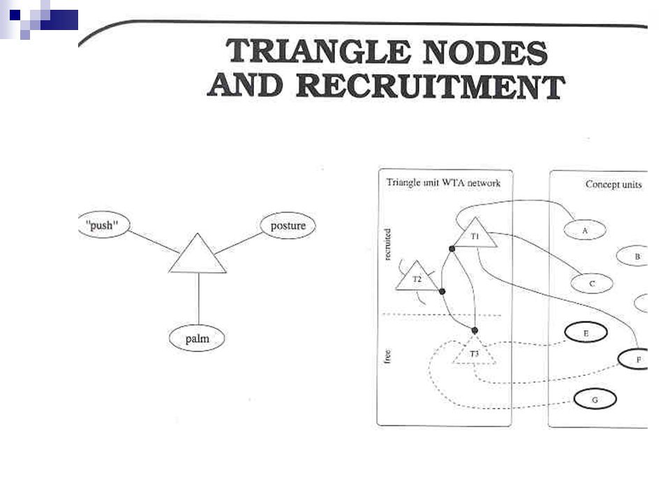
Recruiting connections Given that LTP involves synaptic strength changes and Hebb’s rule involves coincident-activation based strengthening of connections How can connections between two nodes be recruited using Hebbs’s rule?

3
X Y

4
X Y

5
Finding a Connection P = Probability of NO link between X and Y N = Number of units in a “layer” B = Number of randomly outgoing units per unit F = B/N, the branching factor K = Number of Intermediate layers, 2 in the example 0.999.9999.99999 1.367.905.989 210 -440 10 -44 10 -5 N= K= # Paths = (1-P k-1 )*(N/F) = (1-P k-1 )*B P = (1-F) **B**K 10 6 10 7 10 8
*(N/F) = (1-P k-1 )*B P = (1-F) **B**K")
6
Finding a Connection in Random Networks For Networks with N nodes and branching factor, there is a high probability of finding good links. (Valiant 1995)
.")
7
Recruiting a Connection in Random Networks Informal Algorithm 1.Activate the two nodes to be linked 2. Have nodes with double activation strengthen their active synapses (Hebb) 3.There is evidence for a “now print” signal based on LTP (episodic memory)
 3.There is evidence for a now print signal based on LTP (episodic memory).")
10
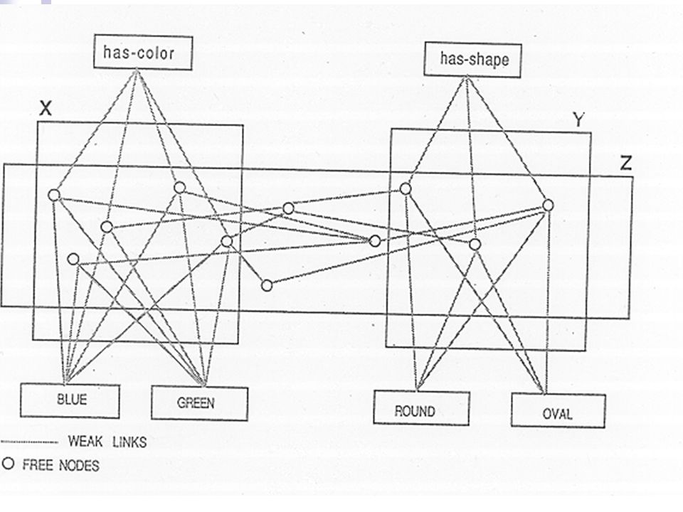
Has-color Green Has-shape Round

11
Has-color Has-shape GREENROUND

12
Hebb’s rule is not sufficient What happens if the neural circuit fires perfectly, but the result is very bad for the animal, like eating something sickening? A pure invocation of Hebb’s rule would strengthen all participating connections, which can’t be good. On the other hand, it isn’t right to weaken all the active connections involved; much of the activity was just recognizing the situation – we would like to change only those connections that led to the wrong decision. No one knows how to specify a learning rule that will change exactly the offending connections when an error occurs. Computer systems, and presumably nature as well, rely upon statistical learning rules that tend to make the right changes over time. More in later lectures.

13
Hebb’s rule is insufficient should you “punish” all the connections? tastebudtastes rotteneats foodgets sick drinks water

14
Models of Learning Hebbian – coincidence Supervised – correction (backprop) Recruitment – one-trial Reinforcement Learning- delayed reward Unsupervised – similarity
 Recruitment – one-trial Reinforcement Learning- delayed reward Unsupervised – similarity")
15
Abbstract Neuron w2w2 wnwn w1w1 w0w0 i 0 =1 o u t p u t y i2i2 inin i1i1... i n p u t i 1 if net > 0 0 otherwise { Threshold Activation Function

16
Boolean XOR input x1 input x2 output 000 011 101 110 h2h2 x2x2 o x1x1 h1h1 1 1.5 AND 1 1 0.5 OR 1 1 0.5 XOR 11

17
Supervised Learning - Backprop How do we train the weights of the network Basic Concepts Use a continuous, differentiable activation function (Sigmoid) Use the idea of gradient descent on the error surface Extend to multiple layers
 Use the idea of gradient descent on the error surface Extend to multiple layers")
18
Backprop To learn on data which is not linearly separable: Build multiple layer networks (hidden layer) Use a sigmoid squashing function instead of a step function.
 Use a sigmoid squashing function instead of a step function.")
19
Tasks Unconstrained pattern classification Credit assessment Digit Classification Speech Recognition Function approximation Learning control Stock prediction

20
Sigmoid Squashing Function w2w2 wnwn w1w1 w0w0 y 0 =1 o u t p u t y2y2 ynyn y1y1... i n p u t

21
The Sigmoid Function x=net y=a

22
The Sigmoid Function x=neti y=a Output=0 Output=1

23
The Sigmoid Function x=net y=a Output=0 Output=1 Sensitivity to input

24
Nice Property of Sigmoids

25
Gradient Descent

26
Gradient Descent on an error

27
Learning as Gradient Descent Error surface for a 2-wt, linear network Complex error surface for hypothetical network training problem

28
Learning Rule – Gradient Descent on an Root Mean Square (RMS) Learn w i ’s that minimize squared error O = output layer
 Learn w i ’s that minimize squared error O = output layer")
29
Gradient Descent Gradient: Training rule:

30
Gradient Descent i2i2 i1i1 global mimimum: this is your goal it should be 4-D (3 weights) but you get the idea
 but you get the idea")
31
Backpropagation Algorithm Generalization to multiple layers and multiple output units

32
Back-Propagation Algorithm We define the error term for a single node to be t i - y i xixi f yjyj w ij yiyi x i = ∑ j w ij y j y i = f(x i ) t i :target Sigmoid:
 t i :target Sigmoid:")
33
Backprop Details Here we go…

34
kji w jk w ij E = Error = ½ ∑ i (t i – y i ) 2 yiyi t i : target The derivative of the sigmoid is just The output layer learning rate
 2 yiyi t i : target The derivative of the sigmoid is just The output layer learning rate")
35
Nice Property of Sigmoids

36
kji w jk w ij E = Error = ½ ∑ i (t i – y i ) 2 yiyi t i : target The hidden layer
 2 yiyi t i : target The hidden layer")
37
Let’s just do an example E = Error = ½ ∑ i (t i – y i ) 2 x0x0 f i1i1 w 01 y0y0 i2i2 b=1 w 02 w 0b E = ½ (t 0 – y 0 ) 2 i1i1 i2i2 y0y0 000 011 101 111 0.8 0.6 0.5 0 0 0.6224 0.5 1/(1+e^-0.5) E = ½ (0 – 0.6224) 2 = 0.1937 0 0 learning rate suppose = 0.5 0.4268
 2 x0x0 f i1i1 w 01 y0y0 i2i2 b=1 w 02 w 0b E = ½ (t 0 – y 0 ) 2 i1i1 i2i2 y0y /(1+e^-0.5) E = ½ (0 – ) 2 = learning rate suppose =")
38
An informal account of BackProp For each pattern in the training set: Compute the error at the output nodes Compute w for each wt in 2 nd layer Compute delta (generalized error expression) for hidden units Compute w for each wt in 1 st layer After amassing w for all weights and, change each wt a little bit, as determined by the learning rate
 for hidden units Compute w for each wt in 1 st layer After amassing w for all weights and, change each wt a little bit, as determined by the learning rate")
39
Backprop learning algorithm (incremental-mode) n=1; initialize w(n) randomly; while (stopping criterion not satisfied and n<max_iterations) for each example (x,d) - run the network with input x and compute the output y - update the weights in backward order starting from those of the output layer: with computed using the (generalized) Delta rule end-for n = n+1; end-while;
 n=1; initialize w(n) randomly; while (stopping criterion not satisfied and n<max_iterations) for each example (x,d) - run the network with input x and compute the output y - update the weights in backward order starting from those of the output layer: with computed using the (generalized) Delta rule end-for n = n+1; end-while;")
40
Backpropagation Algorithm Initialize all weights to small random numbers For each training example do For each hidden unit h: For each output unit k: For each hidden unit h: Update each network weight w ij : with

41
Backpropagation Algorithm “activations” “errors”

42
What if all the input To hidden node weights are initially equal?

43
Momentum term The speed of learning is governed by the learning rate. If the rate is low, convergence is slow If the rate is too high, error oscillates without reaching minimum. Momentum tends to smooth small weight error fluctuations. the momentum accelerates the descent in steady downhill directions. the momentum has a stabilizing effect in directions that oscillate in time.

44
Convergence May get stuck in local minima Weights may diverge …but often works well in practice Representation power: 2 layer networks : any continuous function 3 layer networks : any function

45
Pattern Separation and NN architecture

46
Local Minimum USE A RANDOM COMPONENT SIMULATED ANNEALING

47
Adjusting Learning Rate and the Hessian The Hessian H is the second derivative of E with respect to w. The Hessian, tells you about the shape of the cost surface: The eigenvalues of H are a measure of the steepness of the surface along the curvature directions. a large eigenvalue => steep curvature => need small learning rate the learning rate should be proportional to 1/eigenvalue

48
Overfitting and generalization TOO MANY HIDDEN NODES TENDS TO OVERFIT

49
Stopping criteria Sensible stopping criteria: total mean squared error change: Back-prop is considered to have converged when the absolute rate of change in the average squared error per epoch is sufficiently small (in the range [0.01, 0.1]). generalization based criterion: After each epoch the NN is tested for generalization. If the generalization performance is adequate then stop. If this stopping criterion is used then the part of the training set used for testing the network generalization will not be used for updating the weights.
![Stopping criteria Sensible stopping criteria: total mean squared error change: Back-prop is considered to have converged when the absolute rate of change in the average squared error per epoch is sufficiently small (in the range [0.01, 0.1]).](http://images.slideplayer.com/16/4939169/slides/slide_49.jpg " generalization based criterion: After each epoch the NN is tested for generalization. If the generalization performance is adequate then stop. If this stopping criterion is used then the part of the training set used for testing the network generalization will not be used for updating the weights..")
50
Overfitting in ANNs

51
Early Stopping (Important!!!) Stop training when error goes up on validation set
 Stop training when error goes up on validation set")
52
Stopping criteria Sensible stopping criteria: total mean squared error change: Back-prop is considered to have converged when the absolute rate of change in the average squared error per epoch is sufficiently small (in the range [0.01, 0.1]). generalization based criterion: After each epoch the NN is tested for generalization. If the generalization performance is adequate then stop. If this stopping criterion is used then the part of the training set used for testing the network generalization will not be used for updating the weights.
![Stopping criteria Sensible stopping criteria: total mean squared error change: Back-prop is considered to have converged when the absolute rate of change in the average squared error per epoch is sufficiently small (in the range [0.01, 0.1]).](http://images.slideplayer.com/16/4939169/slides/slide_52.jpg " generalization based criterion: After each epoch the NN is tested for generalization. If the generalization performance is adequate then stop. If this stopping criterion is used then the part of the training set used for testing the network generalization will not be used for updating the weights..")
53
Architectural Considerations What is the right size network for a given job? How many hidden units? Too many: no generalization Too few: no solution Possible answer: Constructive algorithm, e.g. Cascade Correlation (Fahlman, & Lebiere 1990) etc
 etc.")
54
The number of layers and of neurons depend on the specific task. In practice this issue is solved by trial and error. Two types of adaptive algorithms can be used: start from a large network and successively remove some nodes and links until network performance degrades. begin with a small network and introduce new neurons until performance is satisfactory. Network Topology

55
Cascade Correlation It starts with a minimal network, consisting only of an input and an output layer. Minimizing the overall error of a net, it adds step by step new hidden units to the hidden layer. Cascade-Correlation is a supervised learning architecture which builds a near minimal multi-layer network topology. The two advantages of this architecture are that there is no need for a user to worry about the topology of the network, and that Cascade-Correlation learns much faster than the usual learning algorithms.

56
Supervised vs Unsupervised Learning Backprop requires a 'target' how realistic is that? Hebbian learning is unsupervised, but limited in power How can we combine the power of backprop (and friends) with the ideal of unsupervised learning?
 with the ideal of unsupervised learning .")
57
Autoassociative Networks input copy of input as target Network trained to reproduce the input at the output layer Non-trivial if number of hidden units is smaller than inputs/outputs Forced to develop compressed representations of the patterns Hidden unit representations may reveal natural kinds (e.g. Vowels vs Consonants) Problem of explicit teacher is circumvented
 Problem of explicit teacher is circumvented.")
58
Problems and Networks Some problems have natural "good" solutions Solving a problem may be possible by providing the right armory of general-purpose tools, and recruiting them as needed Networks are general purpose tools. Choice of network type, training, architecture, etc greatly influences the chances of successfully solving a problem Tension: Tailoring tools for a specific job Vs Exploiting general purpose learning mechanism

59
Summary Multiple layer feed-forward networks Replace Step with Sigmoid (differentiable) function Learn weights by gradient descent on error function Backpropagation algorithm for learning Avoid overfitting by early stopping
 function Learn weights by gradient descent on error function Backpropagation algorithm for learning Avoid overfitting by early stopping")
60
ALVINN drives 70mph on highways

61
Use MLP Neural Networks when … (vectored) Real inputs, (vectored) real outputs You’re not interested in understanding how it works Long training times acceptable Short execution (prediction) times required Robust to noise in the dataset
 Real inputs, (vectored) real outputs You’re not interested in understanding how it works Long training times acceptable Short execution (prediction) times required Robust to noise in the dataset")
62
Applications of FFNN Classification, pattern recognition: FFNN can be applied to tackle non-linearly separable learning problems. Recognizing printed or handwritten characters, Face recognition Classification of loan applications into credit-worthy and non-credit-worthy groups Analysis of sonar radar to determine the nature of the source of a signal Regression and forecasting: FFNN can be applied to learn non-linear functions (regression) and in particular functions whose inputs is a sequence of measurements over time (time series).
 and in particular functions whose inputs is a sequence of measurements over time (time series)..")
64
Extensions of Backprop Nets Recurrent Architectures Backprop through time

65
Elman Nets & Jordan Nets Updating the context as we receive input In Jordan nets we model “forgetting” as well The recurrent connections have fixed weights You can train these networks using good ol’ backprop Output Hidden ContextInput 1 α Output Hidden ContextInput 1

66
Recurrent Backprop we’ll pretend to step through the network one iteration at a time backprop as usual, but average equivalent weights (e.g. all 3 highlighted edges on the right are equivalent) abc unrolling 3 iterations abc abc abc w2 w1w3 w4 w1w2w3w4 abc
 abc unrolling 3 iterations abc abc abc w2 w1w3 w4 w1w2w3w4 abc.")
Similar presentations


>")


 Reinforcement ~ delayed reward Unsupervised ~ similarity.>")


 –Perceptrons –Feed-forward.>")


>")
