1. Demand Management and FORECASTING Operations Management Dr. Ron Lembke

2. Demand Management Coordinate sources of demand for supply chain to run efficiently, deliver on time Independent Demand ▫Things demanded by end users Dependent Demand ▫Demand known, once demand for end items is known

3. Affecting Demand Increasing demand ▫Marketing campaigns ▫Sales force efforts, cut prices Changing Timing of demand ▫Incentives for earlier or later delivery ▫At capacity, don’t actively pursue more

4. Predicting the Future We know the forecast will be wrong. Try to make the best forecast we can, ▫Given the time we want to invest ▫Given the available data

5. Time Horizons Different decisions require projections about different time periods: Short-range: who works when, what to make each day (weeks to months) Medium-range: when to hire, lay off (months to years) Long-range: where to build plants, enter new markets, products (years to decades)

6. Forecast Impact Finance & Accounting: budget planning Human Resources: hiring, training, laying off employees Capacity: not enough, customers go away angry, too much, costs are too high Supply-Chain Management: bringing in new vendors takes time, and rushing it can lead to quality problems later

7. Qualitative Methods Sales force composite / Grass Roots Market Research / Consumer market surveys & interviews Jury of Executive Opinion / Panel Consensus Delphi Method Historical Analogy - DVDs like VCRs Naïve approach

8. Quantitative Methods Time Series Methods 0. All-Time Average 1. Simple Moving Average 2. Weighted Moving Average 3. Exponential Smoothing 4. Exponential smoothing with trend 5. Linear regression Causal Methods Linear Regression

9. Time Series Forecasting Assume patterns in data will continue, including: Trend (T) Seasonality (S) Cycles (C) Random Variations

10. All-Time Average To forecast next period, take the average of all previous periods Advantages: Simple to use Disadvantages: Ends up with a lot of data Gives equal importance to very old data

11. 4/7/2009 2009 Farm Angels: Ty: 1.000, Jacob 0.833, Noah 0.667 (6 at bats)

12. End of 2009 season

13. Moving Average Compute forecast using n most recent periods Jan Feb MarAprMayJunJul 3 month Moving Avg: June forecast: F Jun = (A Mar + A Apr + A May )/3 If no cycles to demand, quite a bit of freedom to choose n

14. Moving Average Advantages: ▫ Ignores data that is “too” old ▫ Requires less data than simple average ▫ More responsive than simple average Disadvantages: ▫ Still lacks behind trend like simple average, (though not as badly) ▫ The larger n is, more smoothing, but the more it will lag ▫ The smaller n is, the more over-reaction

15. Simple and Moving Averages

16. Centered MA CMA smoothes out variability Plot the average of 5 periods: 2 previous, the current, and the next two Obviously, this is only in hindsight FRB Dalls graphs

17. Centered Moving Average Take average of n periods, Plot the average in the middle period Not useful for forecasting More stable than actuals If seasonality, n = season length (4wks, 12 mo, etc.)

18. CMA - # Periods to Average What if data has 12-month cycle? Ja F M Ap My Jn Jl Au S O N D Ja F M Avg of Jan-Dec gives average of month 6.5: (1+2+3+4+5+6+7+8+9+10+11+12)/12=6.5 Avg of Feb-Jan gives average of month 6.5: (2+3+4+5+6+7+8+9+10+11+12+13)/12=7.5 How get a July average? Average of other two averages

19. Centered Moving Average To center even-number of periods 12: take half each of 1 and 13, plus sum of 2-12. F14 = 0.5 A1 + A2 + A3 + A4 + A5 + A6 + A7 + A8 + A9 + A10 + A11 + A12 + 0.5A13 This is exactly the same as what you get by taking the average of the averages from previous slide

20. Old Data Comparison of simple, moving averages clearly shows that getting rid of old data makes forecast respond to trends faster Moving average still lags the trend, but it suggests to us we give newer data more weight, older data less weight.

21. Weighted Moving Average F Jun = (A Mar + A Apr + A May )/3 = (3A Mar + 3A Apr + 3A May )/9 Why not consider: F Jun = (2A Mar + 3A Apr + 4A May )/9 F Jun = 2/9 A Mar + 3/9 A Apr + 4/9 A May F t = w 1 A t-3 + w 2 A t-2 + w 3 A t-1 Complicated: Have to decide number of periods, and weights for each Weights have to add up to 1.0 Most recent probably most relevant, gets most weight Carry around n periods of data to make new forecast

22. Weighted Moving Average Wts = 0.5, 0.3, 0.2

23. Exponential Smoothing A t-1 Actual demand in period t-1 F t-1 Forecast for period t-1  Smoothing constant >0, <1 Forecast is old forecast plus a portion of the error of the last forecast. Formulas are equivalent, give same answer

24. Exponential Smoothing Smoothing Constant between 0.1-0.3 Easier to compute than moving average Most widely used forecasting method, because of its easy use F 1 = 1,050,  = 0.05, A 1 = 1,000 F 2 = F1 +  (A 1 - F 1 ) = 1,050 + 0.05(1,000 – 1,050) = 1,050 + 0.05(-50) = 1,047.5 units BTW, we have to make a starting forecast to get started. Often, use actual A1

25. Weighted Moving Average Alpha = 0.3

26. Weighted Moving Average Alpha = 0.5

27. Exponential Smoothing We take: And substitute in to get: and if we continue doing this, we get: Older demands get exponentially less weight

28. Choosing  Low  : if demand is stable, we don’t want to get thrown into a wild-goose chase, over-reacting to “trends” that are really just short-term variation High  : If demand really is changing rapidly, we want to react as quickly as possible

29. Averaging Methods Simple Average Moving Average Weighted Moving Average Exponentially Weighted Moving Average (Exponential Smoothing) They ALL take an average of the past ▫With a trend, all do badly ▫Average must be in-between 30 20 10

30. Trend-Adjusted Ex. Smoothing

31. Forecast including trend for period 1 is Suppose actual demand is 115, A 1 =115

32. Trend-Adjusted Ex. Smoothing Forecast including trend for period 1 is Suppose actual demand is 120, A 2 =120

33. Selecting  and  You could: ▫Try an initial value for each parameter. ▫Try lots of combinations and see what looks best. ▫But how do we decide “what looks best?” Let’s measure the amount of forecast error. Then, try lots of combinations of parameters in a methodical way. ▫Let  = 0 to 1, increasing by 0.1  For each  value, try  = 0 to 1, increasing by 0.1

34. Evaluating Forecasts How far off is the forecast? What do we do with this information? Forecasts Demands

35. Evaluating Forecasts Mean Absolute Deviation Mean Squared Error Mean Absolute Percent Error

36. Tracking Signal To monitor, compute tracking signal If >4 or <-4 something is wrong Top should sum to 0 over time. If not, forecast is biased.

37. Monitoring Forecast Accuracy Monitor forecast error each period, to see if it becomes too great 0 -10 10 Forecast Error Forecast Period Lower Limit Upper Limit

38. Updating MAD Simplified calculation avoids keeping running total of all errors and demands: Standard Deviation can be estimated from MAD:

39. Techniques for Trend Determine how demand increases as a function of time t = periods since beginning of data b = Slope of the line a = Value of y t at t = 0

40. Computing Values

41. Linear Regression Three methods ▫Type in formulas for trend, intercept ▫Tools | Data Analysis | Regression ▫Graph, and R click on data, add a trendline, and display the equation. ▫Use intercept(Y,X) and slope(Y,X) commands Fits a trend and intercept to the data. Gives all data equal weight. Exp. smoothing with a trend gives more weight to recent, less to old.

42. Causal Forecasting Linear regression seeks a linear relationship between the input variable and the output quantity. R 2 measures the percentage of change in y that can be explained by changes in x.

43. Video sales of Shrek 2? Shrek did $500m at the box office, and sold almost 50 million DVDs & videos Shrek2 did $920m at the box office

44. Video sales of Shrek 2? Assume 1-1 ratio: ▫920/500 = 1.84 ▫1.84 * 50 million = 92 million videos? ▫Fortunately, not that dumb. January 3, 2005: 37 million sold! March analyst call: 40m by end Q1 March SEC filing: 33.7 million sold. Oops. May 10 Announcement: ▫In 2 nd public Q, missed earnings targets by 25%. ▫May 9, word started leaking ▫Stock dropped 16.7%

45. Lessons Learned Flooded market with DVDs Guaranteed Sales ▫Promised the retailer they would sell them, or else the retailer could return them ▫Didn’t know how many would come back 5 years ago ▫Typical movie 30% of sales in first week ▫Animated movies even lower than that 2004/5 50-70% in first week ▫ Shrek 2: 12.1m in first 3 days ▫American Idol ending, had to vote in first week

46. Washoe Gaming Win, 1993-96 What did they mean when they said it was down three quarters in a row? 1993 1994 1995 1996

47. Seasonality Seasonality is regular up or down movements in the data Can be hourly, daily, weekly, yearly Naïve method ▫N1: Assume January sales will be same as December ▫N2: Assume this Friday’s ticket sales will be same as last

48. Seasonal Factors Seasonal factor for May is 1.20, means May sales are typically 20% above the average Factor for July is 0.90, meaning July sales are typically 10% below the average

49. Seasonality & No Trend SalesFactor Spring200200/250 = 0.8 Summer350350/250 = 1.4 Fall300300/250 = 1.2 Winter150150/250 = 0.6 Total1,000 Avg1,000/4=250

50. Seasonality & No Trend If we expected total demand for the next year to be 1,100, the average per quarter would be 1,100/4=275 Forecast Spring275 * 0.8 = 220 Summer275 * 1.4 = 385 Fall275 * 1.2 = 330 Winter275 * 0.6 = 165 Total1,100

51. Trend & Seasonality Deseasonalize to find the trend 1.Calculate seasonal factors 2.Deseasonalize the demand 3.Find trend of deseasonalized line Project trend into the future 4.Project trend line into future 5.Multiply trend line by seasonal component.

52. Washoe Gaming Win, 1993-96 Looks like a downhill slide -Silver Legacy opened 95Q3 -Otherwise, upward trend 1993 1994 1995 1996 Source: Comstock Bank, Survey of Nevada Business & Economics

53. Washoe Win 1989-1996 Definitely a general upward trend, slowed 93-94

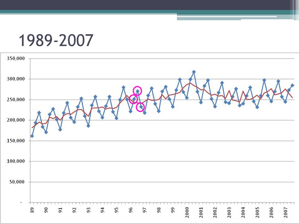
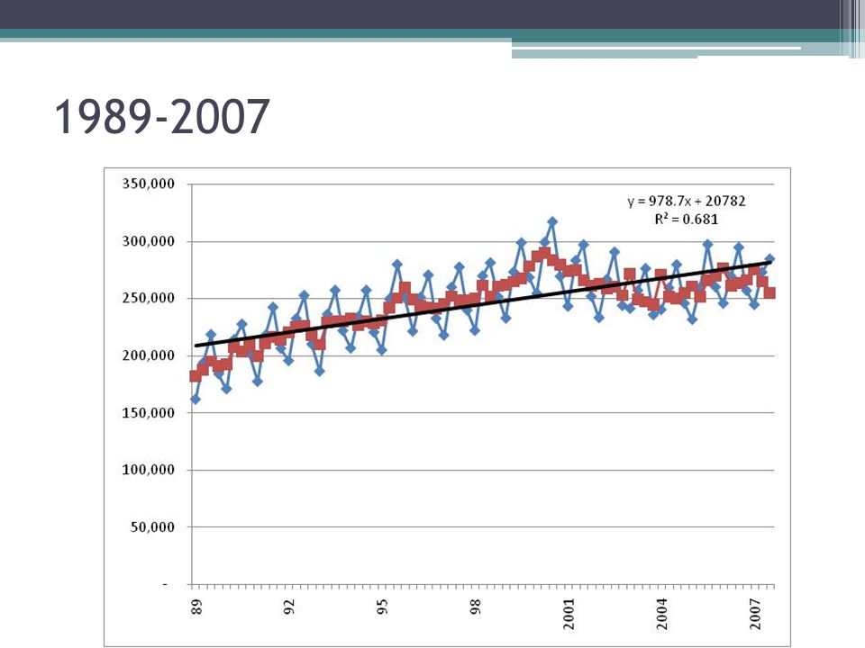
54. 1989-2007

56. 1998-2007 Cache Creek Thunder Valley CC Expands 9/11

57. 2003Q3 - 2007Q3

58. 2003Q2 - 2007Q3

59. 2003-2007 DateQuarterWin 59 276,371 60 235,766 200461 240,221 62 259,350 63 279,758 64 245,811 200565 231,608 66 259,687 67 297,414 68 260,149 200669 245,775 70 269,670 71 294,839 72 257,015 200773 244,643 74 273,116 75 284,734 QAvgIndex 1 240,5620.9168 2 265,4561.0117 3 289,1871.1022 4 254,3250.9693 Total Avg. 262,382 For each Q: Compute Indexes Deseasonalize: Divide Win by Index 276,371 / 1.1022 = 250,755 Compute Avg Win for each Q Divide Avg by Total Avg to get Index: 240,562/262,382 = 0.9168

60. 2003-2007 periodWinDeseasonalized 59 276,371 250,755 60 235,766 243,236 200461 240,221 262,010 62 259,350 256,347 63 279,758 253,828 64 245,811 253,598 200565 231,608 252,616 66 259,687 256,681 67 297,414 269,847 68 260,149 268,391 200669 245,775 268,069 70 269,670 266,548 71 294,839 267,511 72 257,015 265,157 200773 244,643 266,834 74 273,116 269,954 75 284,734 258,343 Do LR on deseasonalized data intercept 185,538.00 slope 1,119.91 rsq 0.497 Create Linear Forecasts Int + slope * period Linear 251,613 252,733 253,853 254,972 256,092 257,212 258,332 259,452 260,572 261,692 262,812 263,932 265,052 266,172 267,291 268,411 269,531 270,651 271,771 272,891 274,011

61. Seasonal Forecast 58 257,062 DeseasonalizedLinearForecast 59 276,371 250,755 251,613 277,317 60 235,766 243,236 252,733 244,972 200461 240,221 262,010 253,853 232,741 62 259,350 256,347 254,972 257,959 63 279,758 253,828 256,092 282,254 64 245,811 253,598 257,212 249,314 200565 231,608 252,616 258,332 236,848 66 259,687 256,681 259,452 262,491 67 297,414 269,847 260,572 287,191 68 260,149 268,391 261,692 253,656 200669 245,775 268,069 262,812 240,956 70 269,670 266,548 263,932 267,023 71 294,839 267,511 265,052 292,129 72 257,015 265,157 266,172 257,998 200773 244,643 266,834 267,291 245,063 74 273,116 269,954 268,411 271,556 75 284,734 258,343 269,531 297,066 76 270,651 262,340 200877 271,771 263,425 78 272,891 264,511 79 274,011 265,596 Multiply Linear forecast by indexes 251,613 * 1.1022 = 277,317 267,291 * 0.9168 = 245,063 QIndex 10.9168 21.0117 31.1022 40.9693

62. Q Win

63. How Good Was It?