1. :By GROUP : Abdul-Majeed et.al
Two-Phase Flow
:By
GROUP : Abdul-Majeed et.al

2. Tow-Phase Flow:
Tow- phase flow in horizontal pipes differs markedly from that in vertical pipes; except for the Beggs and Brill correlation (Beggs and Brill,1973) , which can be applied for any flow direction, completely different correlations are used for horizontal flow than for vertical flow.

3. A : Flow regimes
The flow regime does not affect the pressure drop as significantly in horizontal flow as it dose in vertical flow, because there is no potential energy contribution to the pressure drop in horizontal flow.
The flow regime is considered in some pressure drop correlations and can affect production operations in other ways.
Figure 10-1 (Beggs and Brill, 1973) depicts the commonly described flow regimes in horizontal gas-liquid flow. These can be classified as three types of regimes: segregated flows, in which the two phases are for the most part separate; intermittent flows, in which gas and liquid are alternating; and distributive flows, in which one phase is dispersed in the other phase.

4. : Figure (10-1) :flow regimes in two phase horizontal flow

5. segregated flow is further classified as being stratified smooth, stratified wavy (ripple flow), or annular. At higher gas rates, the interface becomes wavy, and stratified wavy flow results. Annular flow occurs at high gas rates and relatively high liquid rates and consists of an annulus of liquid coating the wall of the pipe and a central core of gas flow, with liquid droplets entrained in the gas.
The intermittent flow regimes are slug flow and plug (also called elongated bubble)flow. Slug flow consists of large liquid slugs alternating with high-velocity bubbles of gas that fill almost the entire pipe. In plug flow, large gas bubbles flow along the top of the pipe.
Distributive flow regimes described in the literature include bubble, mist ,and froth flow.

6. λ= [ (ρg /0.075) (ρL /62.4) ]1/2 Ø= 73/σL [ μL (62.4/ρL )2 ]1/3
Shown in fig. (10-2) The axes for this plot are Gl / λ and Gl λØ / Gg , where Gl and Gg are the mass fluxes of liquid and gas, respectively (lbm/hr-ft2) and the parameters λ and Ø are
λ= [ (ρg /0.075) (ρL /62.4) ]1/2
Ø= 73/σL [ μL (62.4/ρL )2 ]1/3
Where densities are in lbm/ft3 , μ is in cp, and σl is in dynes/cm.

8. NFr= um2 / g D The Beggs and Brill correlation :
is based on a horizontal flow regime map that divides the domain into the three flow regime categories, segregated, intermittent and distributed. This map, shown in Fig. 10-4, plots the mixture Froude number defined as
NFr= um2 / g D
Versus the input liquid fraction, λl.

9. Taitel and Dukler (1976):
developed a theoretical model of the flow regime transitions in horizontal gas-liquid flow; their model can be used to generate flow regime maps for particular fluids and pipe size. Figure shows a comparison of their flow regime prediction with those of Mandhane et al. for air-water flow in a 2.5-cm pipe.

11. Example:
Using the Baker, mandhane, and Beggs and Brill flow regime maps, determine the flow regime for the flow of qo= 2000 bbl/day of oil and qg= 1MM scf/day of gas at 800 psia and 1750F in a 2-1/2 in. I.D. pipe. The fluids are Given:
-for liquid: ρ=49.92 lbm/ft3 ; μl=2 cp ;
σl=30 dynes/cm; ql=0.130 ft3/sec.
-for gas: ρ=2.61 lbm/ft3 ; μg= cp ;
Z=0.935 ; qg=0.242 ft3/sec.

12. Solution: -cross sectional are = (π/4)*(D/12)2
-cross sectional are = (π/4)*(D/12)2
=(π/4)*(2.5/12)2= ft2
usl= ql/A = 0.13/ =3.812 ft/sec
usg= qg/A =0.242/0.0341=7.1 ft/sec
go to fig.(10-3): the flow regime is predicted to
be slug flow.
um= usl+usg= 10.9 ft/sec

13. for using Baker map, we calculation: Gl, Gg, λ, and Ø.
Gl= usl ρl= 3.81(ft/sec) * 49.92(lbm/ft3) * 3600(sec/hr)
= 6.84* 105 lbm/hr-ft2
Gg= usgρg= 7.11(ft/sec) * 2.6(lbm/ft3) * 3600(sec/hr)
= 6.65* 104 lbm/hr-ft2
λ =[(2.6/0.075)(49.92/62.4)]1/2 = 5.27
Ø =(73/30)[2(62.4/49.92)2]1/3 = 3.56
The coordinates for the baker map are
Gg/λ =(6.65*104)/5.27 = 1.26*104
GlλØ/Gg= (6.84*105)(5.27)(3.56)/(6.65*104)= 193
Reading from fig. 10-2, the flow regime is predicted to be dispersed bubble, though the conditions are very near the boundaries with slug flow and annular mist flow.

15. For using Beggs and Brill, calculation NFr , λl .
NFr= (10.9 ft/sec)2/(32.17ft/sec2)[(2.5/12)ft]
=17.8
λl =usl/um
=3.81/10.9
= 0.35
From fig. (10-4): the flow regime is predicted to be intermittent.

17. :B: Pressure gradient correlations
Begs and brill correlation: The Beggs and Brill correlation presented in applied to horizontal flow. The correlation is somewhat simplified, since the angle Ѳ is 0, making the factor ψ equal to 1. This correlation is presented in section
∆Ptotal=∆Pf+∆Pel

18. Eaton correlation: The Eaton correlation (Eaton et al
Eaton correlation: The Eaton correlation (Eaton et al., 1967) was developed empirically from a series of tests in 2-in.- and 4-in.-diameter, 1700-ft-long lines. It consists primarily of correlations for liquid holdup and friction factor.
The friction factor( f ) is obtained from the correlation shown in Fig as a function of the mass flow rate of the liquid, ml, and the total mass flow rate, mm' For the constant given in this figure to compute the abscissa, mass flow rates are in Ibm/sec, diameter is in ft, and viscosity is in lbm/ft- sec.

19. :Example 7.5
Two gas-condensate wells feed into a 4-in. gathering line 2.10 mi long. Well A will flow at the rate of 3 MMcfd, and well B will flow at the rate of 1 MMcfd. The following data are available on each well:

20. * Gallons per Mcf of gas The
summation of the uphill rises in the line is 143 ft. The initial pressure at the wells is 900 psig What is the pressure drop in the line?

21. SOLUTION: Gas: Line diameter = = 0.6667 ft.
Line length = 5 × 5280 = ft.
= Mcf/hr.
Assume an average pressure in the pipeline of 1350 psig or 1365 psia.
Assume an average temperature in the pipeline of 60 °F or 520 °R.
Calculate the weighted average specific gravity of the commingled gas stream:
= 0.67
Calculate the gas viscosity. The molecular weight of the gas is:
Ma = γg × = 0.67 × =
From Fig.(2.10) μ1 = cp.

23. = × 0.67 = 376 °R.
= – 58.7 × 0.67 = 670 psia. = =
From Fig. (2.11) μ/μ1 = 1.36
Calculate the gas viscosity at pipeline conditions:
= cp.
From Fig. 2.4, Z = 0.755

25. Calculate the gas volume at pipeline conditions:
=6.776 Mcf/hr = 6776 ft3/hr.
Calculate the density of the gas at pipeline conditions:
= Lbm/ft3.

26. Liquid:
Assume that the average composition of the condensate is normal octane (n-C8H18).
From Table( 2-2):Tpc = °R, Ppc = psia, Ma = and γL = 0.65.
=0.65 × 62.4 = lbm/ft3
=0.9216
= 3.785

28. From Fig. (7.11)
= cp.
From a plot of GPM vs. pressure (Fig. 7.17), the GPM at psig is 4 for well A , for well B and for well C:
QLPL = × × × = gal/day = ft3/hr
1 gal/day = cuf/hr

31. Two-phase: 1 cuf / hr = 0.0002778 cuf / sec
Calculate λ, the input liquid-volume ratio: =
Calculate , the mixture velocity:
= ft3/hr
= ft/s.
Calculate , the mixture velocity:
= cp = Lbm/ft-s
1 cuf / hr = cuf / sec

32. # Now, calculate the two-phase Reynolds number
# Now, calculate the two-phase Reynolds number. This is a trial and error calculation. Assume a value for , the liquid hold-up.
Assume :
Calculate , the two-phase density:
= Lbm/ft3.

33. =
From Fig. (7.15) : This is not a close enough check, and the calculation must be repeated with the
new value of

35. = Lbm/ft3. =
From Fig.( 7.15) : This checks.
Calculate the single-phase friction factor: =

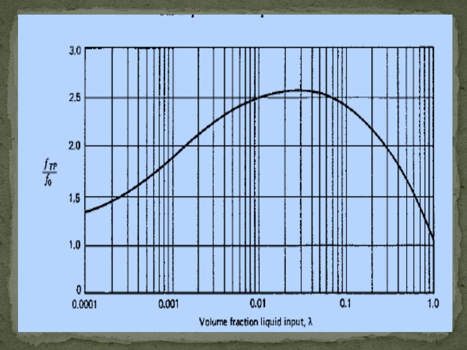
36. Determine the friction factor ratio
from Fig. (7.14):
Calculate the two-phase friction factor: =
Calculate the pressure drop due to friction:
= psi

38. Next, the pressure drop due to elevation changes must be considered.
Calculate VSG , then superficial gas velocity:
= ft3/hr = ft3/s.
From Fig. (7.16):
Calculate the elevation pressure drop:
= psi
Calculate the total pressure drop:
= psi.

41. example two phase not found in.
THANK
YOU
FOR ALL
note:
example two phase not found in.