Download presentation
Presentation is loading. Please wait.

1
AMA522 SCHEDULING Set # 2 Dr. LEE Heung Wing Joseph
Phone: Office : HJ639 AMA522 Scheduling

2
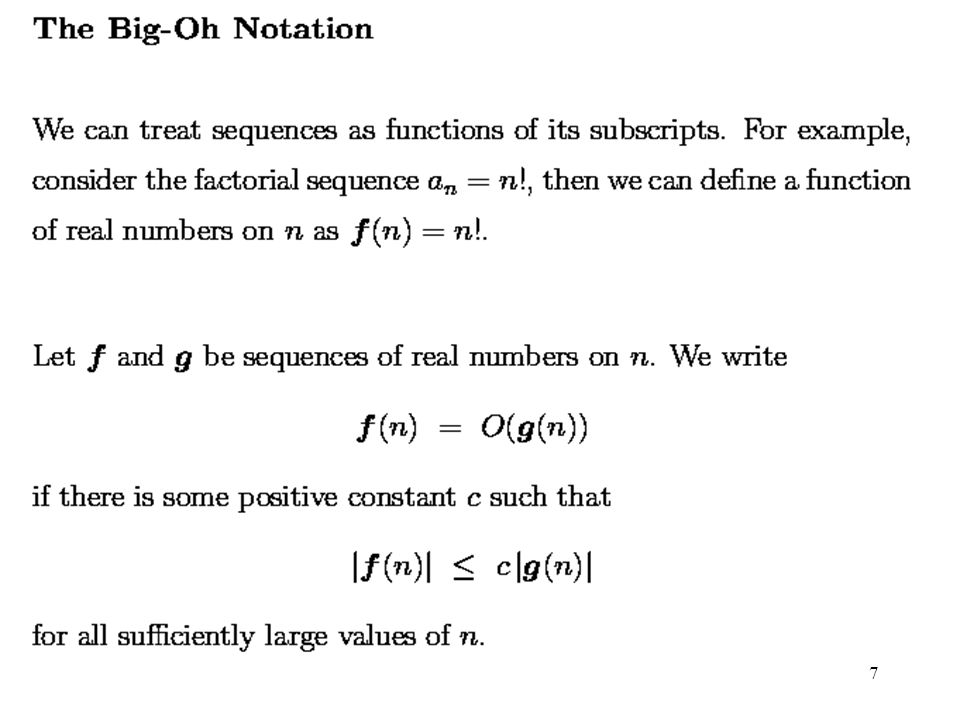
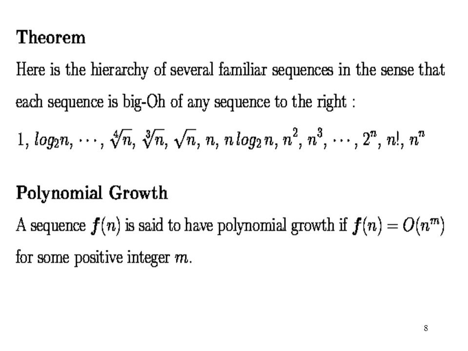
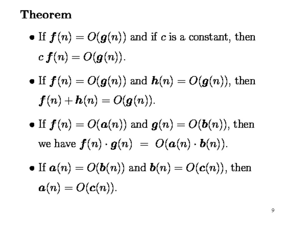
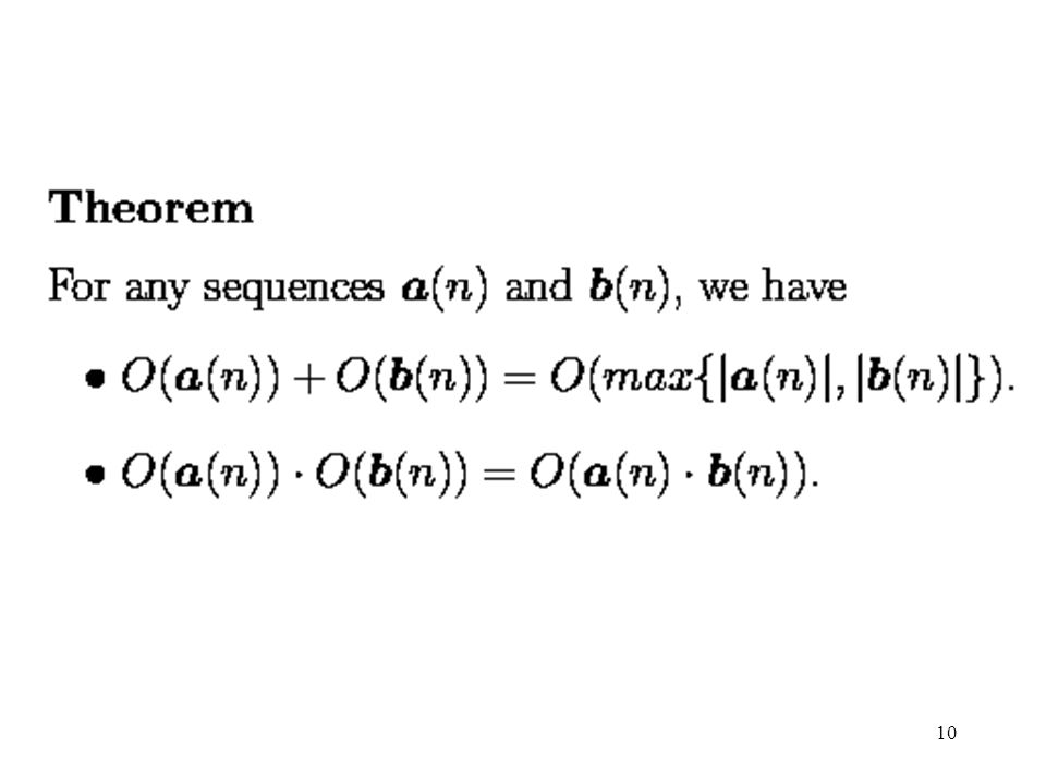
Complexity Theory Classic scheduling theory draws heavily on complexity theory The complexity of an algorithm is its running time in terms of the input parameters (e.g., number of jobs and number of machines) Big-Oh notation, e.g., O(n2m)
 Big-Oh notation, e.g., O(n2m)")
11
P and NP problems The efficiency of an algorithm for a given problem is measured by the maximum (worst-case) number of computational steps needed to obtain an optimal solution as a function of the size of the instance. Problems which have a known polynomial algorithm are said to be in class P. These are problems for which an algorithm is known to exist and it will stop on the correct output while effort is bounded by a polynomial function of the size of the problem. For NP (non-deterministic polynomial problems) no simple algorithm yields optimal solutions in a limited amount of computer time.
 number of computational steps needed to obtain an optimal solution as a function of the size of the instance. Problems which have a known polynomial algorithm are said to be in class P. These are problems for which an algorithm is known to exist and it will stop on the correct output while effort is bounded by a polynomial function of the size of the problem. For NP (non-deterministic polynomial problems) no simple algorithm yields optimal solutions in a limited amount of computer time.")
12
Polynomial versus NP-Hard

13
Scheduling in Practice
Practical scheduling problems cannot be solved this easily! Need: Heuristic algorithms Knowledge-based systems Integration with other enterprise functions However, classic scheduling results are useful as a building block

14
General Purpose Scheduling Procedures
Some scheduling problems are easy Simple priority rules Complexity: polynomial time However, most scheduling problems are hard Complexity: NP-hard, strongly NP-hard Finding an optimal solution is infeasible in practice heuristic methods

15
Types of Heuristics Simple Dispatching Rules
Composite Dispatching Rules Branch and Bound Beam Search Simulated Annealing Tabu Search Genetic Algorithms Construction Methods Improvement

16
Single Machine Deterministic Models
Jobs: J1, J2, ..., Jn Assumptions: The machine is always available throughout the scheduling period. The machine cannot process more than one job at a time. Each job must spend on the machine a prescribed length of time.

17
S(t) 3 2 1 t J2 J3 J1 ...
 t J2 J3 J1 ...")
18
Requirements that may restrict the feasibility of schedules:
precedence constraints no preemptions release dates deadlines Whether some feasible schedule exist? NP hard Objective function f is used to compare schedules. f(S) < f(S') whenever schedule S is considered to be better than S' problem of minimising f(S) over the set of feasible schedules.
 < f(S ) whenever schedule S is considered to be better than S problem of minimising f(S) over the set of feasible schedules.")
19
1. Completion Time Models
Due date related objectives: 2. Lateness Models 3. Tardiness Models 4. Sequence-Dependent Setup Problems

20
Completion Time Models
Contents 1. An algorithm which gives an optimal schedule with the minimum total weighted completion time 1 || wjCj 2. An algorithm which gives an optimal schedule with the minimum total weighted completion time when the jobs are subject to precedence relationship that take the form of chains 1 | chain | wjCj

21
1 || wjCj Theorem (3.1.1). The weighted shortest processing time first rule (WSPT) is optimal for 1 || wjCj WSPT: jobs are ordered in decreasing order of wj/pj The next follows trivially: The problem 1 || Cj is solved by a sequence S with jobs arranged in nondecreasing order of processing times.

22
Proof. By contradiction. S is a schedule, not WSPT, that is optimal.
j and k are two adjacent jobs such that which implies that wj pk < wk pj S: ... j k ... t t + pj + pk S’ ... ... k j t t + pj + pk S: (t+pj) wj + (t+pj+pk) wk = t wj + pj wj + t wk + pj wk pk wk S’: (t+pk) wk + (t+pk+pj) wj = t wk + pk wk + t wj + pk wj pj wj the completion time for S’ < completion time for S contradiction!
 wj + (t+pj+pk) wk = t wj + pj wj + t wk + pj wk + pk wk. S’: (t+pk) wk + (t+pk+pj) wj = t wk + pk wk + t wj + pk wj + pj wj. the completion time for S’ < completion time for S contradiction!")
23
1 | chain | wjCj chain 1: 1 2 ... k chain 2: k+1 k+2 ... n Lemma If the chain of jobs 1,...,k precedes the chain of jobs k+1,...,n.

24
Proof: Under the sequence 1,…,k, k+1, …, n, say S,
the total weighted completion time of S is given by ………(*)
")
25
Under the sequence k+1, …, n, 1,…,k,, say S’,
the total weighted completion time is given by ………(**)
")
26
By comparing the total weighted completion time S and S’,
We have (*) < (**) only if
 < (**) only if.")
27
Let l* satisfy factor of chain 1,...,k l* is the job that determines the factor of the chain Note that for

28
Note also that for ………(***) The reason is not hard to see. Suppose a,b,c,d > 0, and Then, by cross multiplication, we have which is Thus, we have

29
Lemma 3.1.3. If job l* determines (1,...,k) , then there exists an
optimal sequence that processes jobs 1,...,l* one after another without interruption by jobs from other chains. Proof: By Contradiction. Suppose the optimal sequence is 1,…,u, v, u+1, …, l*, say S. Let S’ be the sequence v,1,…,u, u+1, …, l*, and let S’’ be the sequence 1,…,u, u+1, …, l*,v.

30
The total weighted completion time of S is less than S’ , then
by Lemma 3.1.2, we have The total weighted completion time of S is less than S’’ , then by Lemma 3.1.2, we have

31
Job l* is the job that determines the factor of the chain (1,...,k)
then by (***), we have If S is better than S’’, then Therefore, S’ is better than S !!!
, we have. If S is better than S’’, then. Therefore, S’ is better than S !!!")
32
Similarly, if S is better than S’, then
Therefore, S’’ is better than S !!! Algorithm Whenever the machine is free, select among the remaining chains the one with the highest factor. Process this chain up to and including the job l* that determines its factor.

33
Example chain 1: 1 2 3 4 chain 2: 5 6 7 factor of chain 1 is determined by job 2: (6+18)/(3+6)=2.67 factor of chain 2 is determined by job 6: (8+17)/(4+8)=2.08 chain 1 is selected: jobs 1, 2 factor of the remaining part of chain 1 is determined by job 3: 12/6=2 factor of chain 2 is determined by job 6: 2.08 chain 2 is selected: jobs 5, 6
/(4+8)=2.08. chain 1 is selected: jobs 1, 2. factor of the remaining part of chain 1 is determined by job 3: 12/6=2. factor of chain 2 is determined by job 6: chain 2 is selected: jobs 5, 6.")
34
factor of the remaining part of chain 1 is determined by job 3: 2
chain 1 is selected: job 3 factor of the remaining part of chain 1 is determined by job 4: 8/5=1.6 factor of the remaining part of chain 2 is determined by job 7: 1.8 chain 2 is selected: job 7 job 4 is scheduled last the final schedule: 1, 2, 5, 6, 3, 7, 4

35
1 | prec | wjCj Polynomial time algorithms for the more complex precedence constraints than the simple chains are developed. The problems with arbitrary precedence relation are NP hard. 1 | rj, prmp | wjCj Try the preemptive version of the WSPT rule: At any point in time, the available job with the highest ratio of weight to remaining processing time is selected for processing. The priority level of job increases while being processed, and therefore not be preempted by another job already available at the start of its processing. The preemtive version of the WSPT rule does not always lead to an optimal solution, and the problem is NP hard.

36
1 | rj, prmp | Cj preemptive version of the SPT rule is optimal
1 | rj | Cj is NP hard

37
Summary 1 || wjCj WSPT rule
1 | chain | wjCj a polynomial time algorithm is given 1 | prec | wjCj with arbitrary precedence relation is NP hard 1 | rj, prmp | wjCj the problem is NP hard 1 | rj, prmp | Cj preemptive version of the SPT rule is optimal 1 | rj | Cj is NP hard

38
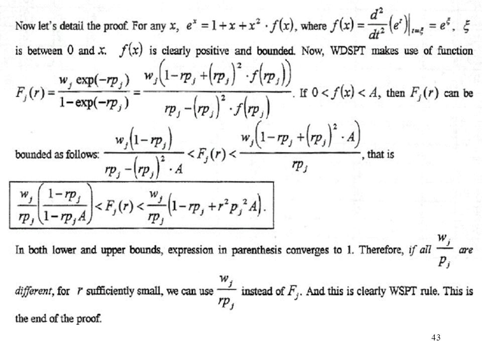
Consider 1 | | wj(1-e-rCj)
where r is the discount rate Scheduled in the decreasing order of This rule is referred to as the Weighted Discounted Shortest Processing Time first (WDSPT) rule.
 rule.")
39
Theorem. The WDSPT is optimal for 1 | | wj(1-e-rCj).
Proof. By contradiction. S is a schedule, not WDSPT, is optimal. Jobs j and k are two adjacent jobs such that S: ... j k t t + pj + pk S’ ... ... k j t t + pj + pk The Cost for S :

40
The Cost for S’ : , so But Rearrange it, we have Thus Hence

41
By adding wj+wk to both sides of the inequality, we have
Factorizing wj and wk , we then have Therefore, cost for S’ is less than that of S !!!

42
Assume that not equal to for all j and k.
Ex3.11 Consider 1 | | wj(1-e-rCj). Assume that not equal to for all j and k. Show that for r sufficiently close to zero, the optimal sequence is WSPT.
. Assume that not equal to for all j and k. Show that for r sufficiently close to zero, the optimal sequence is WSPT.")
45
Lawler’s Algorithm Backward algorithm which gives an optimal schedule for 1 | prec | hmax hmax = max ( h1(C1), ... ,hn(Cn) ) hj are nondecreasing cost functions Notation makespan Cmax = pj completion of the last job Let J be the set of jobs already scheduled they have to be processed during the time interval JC = complement of set J, set of jobs still to be scheduled J' JC set of jobs that can be scheduled immediately before set J (schedulable jobs)
")
46
Lawler’s Algorithm for 1 | | hmax
Step 1. J = JC = {1,...,n} k = n Step 2. Let j* be such that Place j* in J in the k-th order position Delete j* from JC Step 3. If JC = then Stop else k = k - 1 go to Step 2

47
Example 3.2.3 (no precedence relationships between jobs)
J = JC={1, 2, 3} jobs still to be scheduled p1+p2+p3=10 h1(10) = 11 h2(10) =12 h3(10) =10 Job 3 is scheduled last and has to be processed in [5, 10]. 10 5 ... 3
 = 11. h2(10) =12. h3(10) =10. Job 3 is scheduled last and has to be processed in [5, 10]")
48
J = {3} JC={1, 2} jobs still to be scheduled
p1+p2= 5 h1(5) = 6 h2(5) = 6 Either job 1 or job 2 may be processed before job 3. 10 5 3 2 1 or 10 5 3 1 2 Two schedules are optimal: 1, 2, 3 and 2, 1, 3
 = 6. h2(5) = 6. Either job 1 or job 2 may be processed before job or Two schedules are optimal: 1, 2, 3 and 2, 1, 3.")
49
Lawler’s Algorithm (3.2.1) for 1 | prec | hmax
Step 1. J = , JC = {1,...,n} J' the set of all jobs with no successors k = n Step 2. Let j* be such that Place j* in J in the k-th order position Delete j* from JC Modify J' to represent the set of jobs which can be scheduled immediately before set J. Step 3. If JC = then Stop else k = k - 1 go to Step 2

50
Example. What will happen in the previous example if the precedence 1 2 has to be taken into account? J = JC={1, 2, 3} still to be scheduled J'={2, 3} have no successors p1+p2+p3= 10 h2(10) = 12 h3(10) = 10 J = {3} JC={1, 2} still to be scheduled J'={2} can be scheduled immediately before J p1+p2= 5 h2(5) = 6 J = {3, 2} JC={1} J'={1} h1(2) = 3 Optimal schedule: 1, 2, hmax = 10 10 5 ... 3 10 5 3 2 10 5 3 2 1 2
 = 12. h3(10) = 10. J = {3} JC={1, 2} still to be scheduled J ={2} can be scheduled immediately before J. p1+p2= 5. h2(5) = 6. J = {3, 2} JC={1} J ={1} h1(2) = 3. Optimal schedule: 1, 2, 3. hmax =")
51
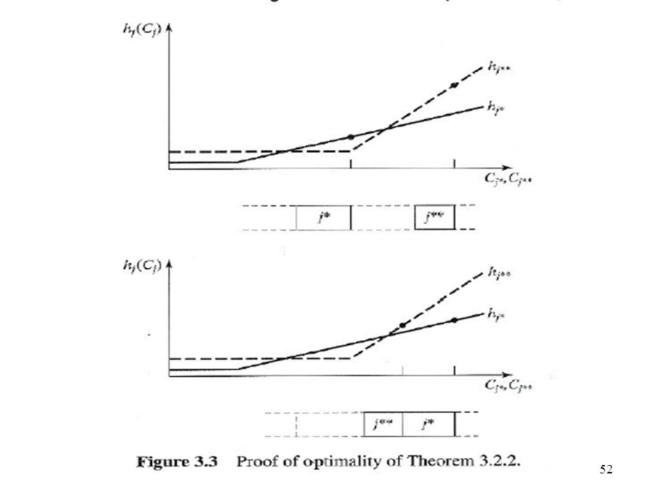
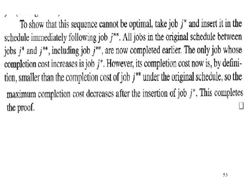
Theorem 3.2.2 Algorithm (3.2.1) yields an optimal schedule for 1 | prec | hmax
 yields an optimal schedule for 1 | prec | hmax")
54
The worst case computation time required by this algorithm can be established as follows.
There are n steps needed to schedule the n jobs. At each step at most n jobs have to be considered. The overall running time of the algorithm is therefore bounded by O(n2).
.")
55
1 || Lmax is the special case of the 1 | prec | hmax
where hj = Cj - dj algorithm results in the schedule that orders jobs in increasing order of their due dates - earliest due date first rule (EDD)
")
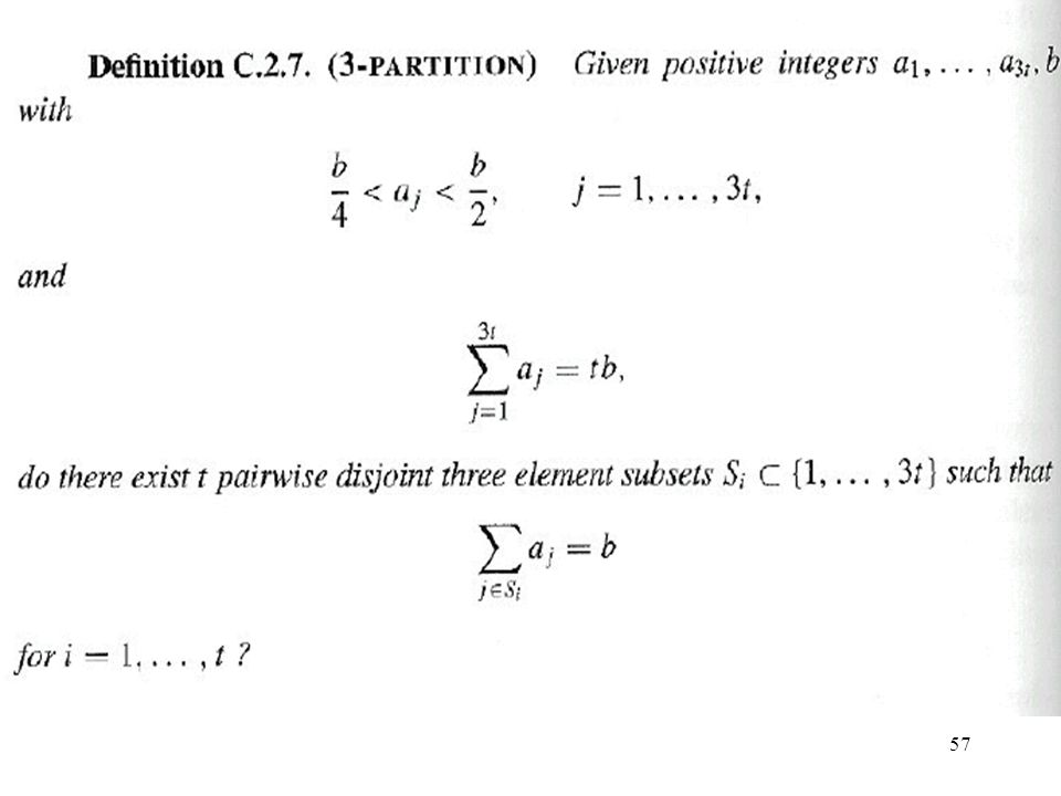
56
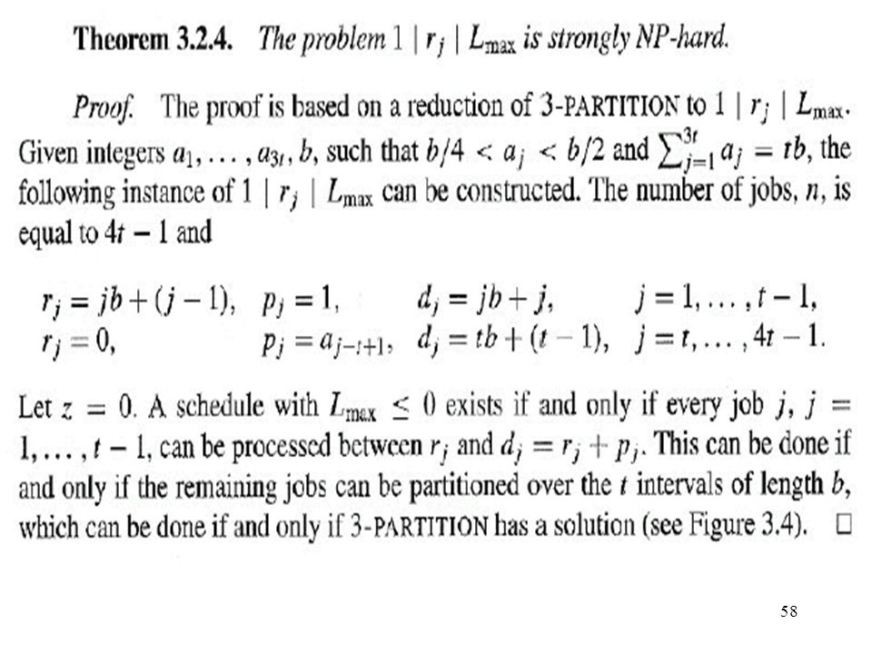
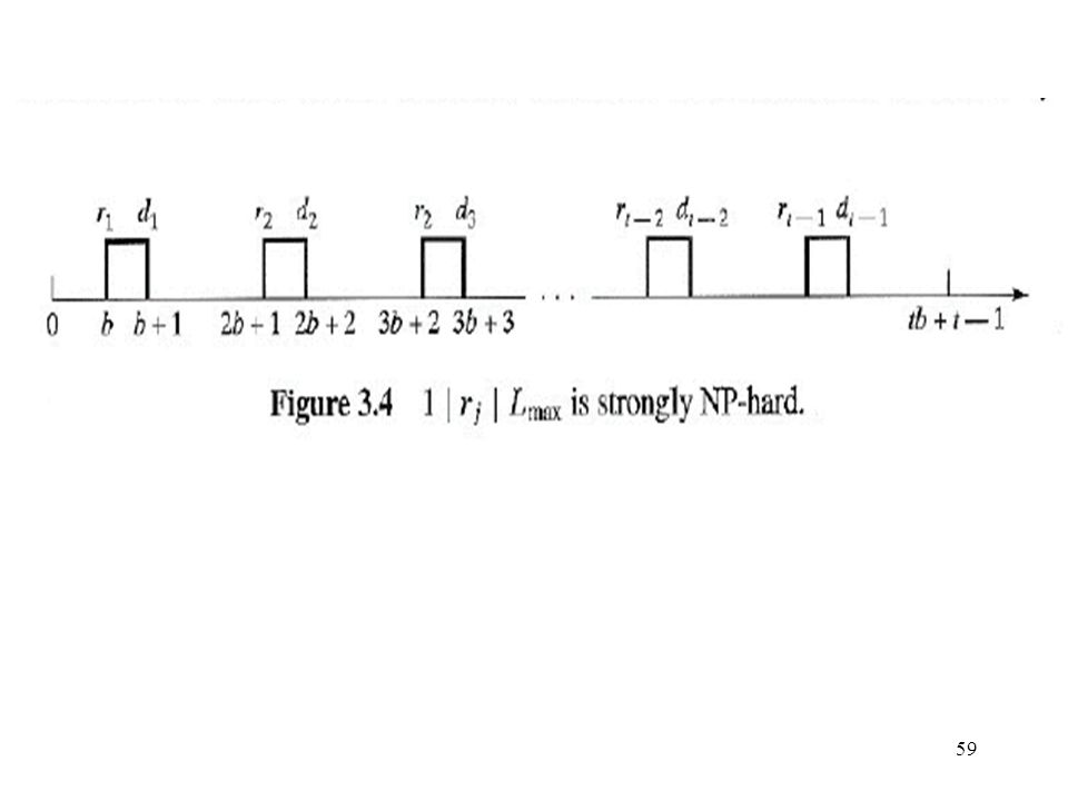
1 | rj | Lmax is NP hard , branch-and-bound is used
1 | rj , prec | Lmax similar branch-and-bound Solution space contains n! schedules (n is number of jobs). Total enumeration is not viable !
. Total enumeration is not viable !")
60
Branch and Bound The problem
cannot be solved using a simple dispatching rule so we will try to solve it using branch and bound To develop a branch and bound procedure: Determine how to branch Determine how to bound

61
Example Data

62
Branching (•,•,•,•) (1,•,•,•) (2,•,•,•) (3,•,•,•) (4,•,•,•)
 (1,•,•,•) (2,•,•,•) (3,•,•,•) (4,•,•,•)")
63
k-1 level, j1, ... , jk-1 are scheduled,
*,*,*,* 1,*,*,* 2,*,*,* n,*,*,* 1,2,*,* 1,3,*,* . . . 1st level 2nd level Branching rule: k-1 level, j1, ... , jk-1 are scheduled, jk need to be considered if no job still to be scheduled can not be processed before the release time of jk that is: J set of jobs not yet scheduled t is time when jk-1 is completed

64
Branching (•,•,•,•) (1,•,•,•) (2,•,•,•) (3,•,•,•) (4,•,•,•)
Discard immediately because

65
Job # 1 Job # 2 Job # 4 Job # 1 Job # 2 Job # 3

66
Branching (•,•,•,•) (1,•,•,•) (2,•,•,•) (3,•,•,•) (4,•,•,•)
Need to develop lower bounds on these nodes and do further branching.

67
Bounding (in general) Typical way to develop bounds is to relax the original problem to an easily solvable problem Three cases: If there is no solution to the relaxed problem there is no solution to the original problem If the optimal solution to the relaxed problem is feasible for the original problem then it is also optimal for the original problem If the optimal solution to the relaxed problem is not feasible for the original problem it provides a bound on its performance

68
Relaxing the Problem The problem is a relaxation to the problem
Not allowing preemption is a constraint in the original problem but not the relaxed problem We know how to solve the relaxed problem (preemptive EDD rule)
")
69
Sub Example for non-preemtive vs preemtive schedules.
Non-preemptive schedules L1=3 L2=6 Lmax=6 1 2 3 7 12 2 1 5 9 L1=5 L2=-1 Lmax=5 Preemptive schedule obtained using EDD L1=3 L2=3 Lmax=3 2 1 3 7 9 the lowest Lmax !

70
Bounding Preemptive EDD rule optimal for the preemptive version of the problem Thus, solution obtained is a lower bound on the maximum delay If preemptive EDD results in a non-preemptive schedule all nodes with higher lower bounds can be discarded.

71
Lower Bounds Start with (1,•,•,•): Job with EDD is Job 4 but
Second earliest due date is for Job 3 Job 1 Job 2 Job 3 Job 4

72
Branching (•,•,•,•) (1,•,•,•) (2,•,•,•) (3,•,•,•) (4,•,•,•) (1,2,•,•)
(1,3,•,•) (1,3,4,2)
 (1,3,4,2)")
73
*, *, *, * 1,*,*,* 1 [0, 4] L1=-4 3 [4, 5] 4 [5, 10] L4=0 3 [10, 15] L3=4 2 [15, 17] L2=5 2,*,*,* 2 [1, 3] L2=-9 1 [3, 7] L1=-1 4 [7, 12] L4=2 3 [12, 18] L3=7 4,*,*,* either job 1 or 2 can be processed before 4 ! 3,*,*,* job 2 can be processed before 3 ! 1,2,*,* 1 [0, 4] L1=-4 2 [4, 6] L2=-6 4 [6, 11] L4=1 3 [11, 17] L3=6 1,3,*,* 1 [0, 4] L1=-4 3 [4, 10] L3=-1 4 [10, 15] L4=5 2 [15, 17] L3=5 Schedule: 1, 3, 4, 2,
![*, *, *, * 1,*,*,* 1 [0, 4] L1=-4. 3 [4, 5] 4 [5, 10] L4=0. 3 [10, 15] L3=4. 2 [15, 17] L2=5. 2,*,*,*](http://slideplayer.com/slide/4792144/15/images/73/%2A%2C+%2A%2C+%2A%2C+%2A+1%2C%2A%2C%2A%2C%2A+1+%5B0%2C+4%5D+L1%3D-4.+3+%5B4%2C+5%5D+4+%5B5%2C+10%5D+L4%3D0.+3+%5B10%2C+15%5D+L3%3D4.+2+%5B15%2C+17%5D+L2%3D5.+2%2C%2A%2C%2A%2C%2A.jpg "2 [1, 3] L2=-9. 1 [3, 7] L1=-1. 4 [7, 12] L4=2. 3 [12, 18] L3=7. 4,*,*,* either job 1 or 2 can be processed before 4 ! 3,*,*,* job 2 can be processed before 3 ! 1,2,*,* 1 [0, 4] L1=-4. 2 [4, 6] L2=-6. 4 [6, 11] L4=1. 3 [11, 17] L3=6. 1,3,*,* 1 [0, 4] L1=-4. 3 [4, 10] L3=-1. 4 [10, 15] L4=5. 2 [15, 17] L3=5. Schedule: 1, 3, 4, 2,")
74
Summary 1 | prec | hmax , hmax=max( h1(C1), ... ,hn(Cn) ), Lawler’s algorithm 1 || Lmax EDD rule 1 | rj | Lmax is NP hard , branch-and-bound is used 1 | rj , prec | Lmax similar branch-and-bound 1 | rj, prmp | Lmax preemptive EDD rule

75
Tardiness Models Contents
1. Moor’s algorithm which gives an optimal schedule with the minimum number of tardy jobs 1 || Uj 2. An algorithm which gives an optimal schedule with the minimum total tardiness 1 || Tj Literature: Scheduling, Theory, Algorithms, and Systems, Michael Pinedo, Prentice Hall, 1995, Chapters 3.3 and 3.4 or new: Second Addition, 2002, Chapter 3.

76
Moor’s algorithm for 1 || Uj
Optimal schedule has this form jd1,...,jdk, jt1,...,jtl meet their due dates EDD rule do not meet their due dates Notation J set of jobs already scheduled JC set of jobs still to be scheduled Jd set of jobs already considered for scheduling, but which have been discarded because they will not meet their due date in the optimal schedule

77
Step 1. J = Jd = JC = {1,...,n} Step 2. Let j* be such that Add j* to J Delete j* from JC Step 3. If then go to Step 4. else let k* be such that Delete k* from J Add k* to Jd Step 4. If Jd = STOP else go to Step 2.

78
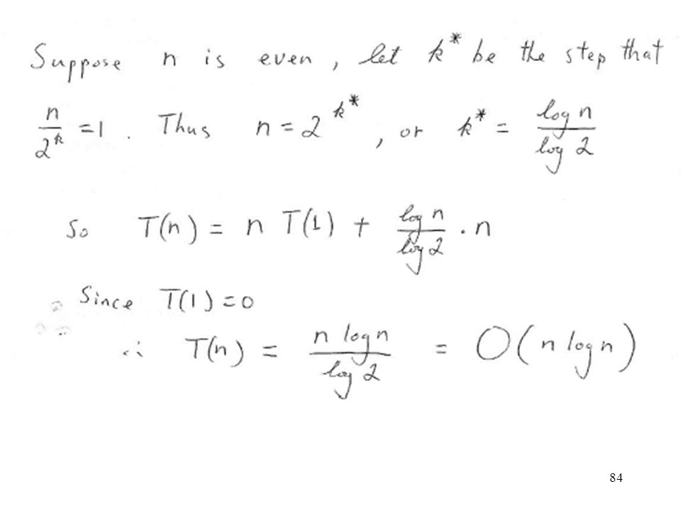
Since the algorithm basically orders the jobs according to their due dates, the worst case computation time is that of a simple sort, that is, O(n log(n)). What is a simple Sort ?? O(n log(n)) ??? Let’s investigate a method called Mergesort.
) Let’s investigate a method called Mergesort.")
79
Description of MergeSort
MergeSort is a recursive sorting procedure that uses O(n log n) comparisons in the worst case. To sort an array of n elements, we perform the following three steps in sequence: If n<2 then the array is already sorted. Stop now. Otherwise, n>1, and we perform the following three steps in sequence: Sort the left half of the the array. Sort the right half of the the array. Merge the now-sorted left and right halves
 comparisons in the worst case. To sort an array of n elements, we perform the following three steps in sequence: If n<2 then the array is already sorted. Stop now. Otherwise, n>1, and we perform the following three steps in sequence: Sort the left half of the the array. Sort the right half of the the array. Merge the now-sorted left and right halves.")
80
Time bounds To get an idea of how long MergeSort takes, we count the number of comparisons it makes in the worst case. Call this function M(n). We parameterize it by the size of the array, n, because MergeSort takes longer on longer inputs. It is difficult to describe M(n) exactly, so instead we describe a simpler function T(n) which bounds M(n) from above, i.e. M(n) <= T(n). An expression for T(n) Because MergeSort has two cases, the description of T also has two cases. The base case is just T(n) = 0, if n<2. The induction case says that the number of comparisons used to sort n items is at most the sum of the worst-case number of comparisons for each of the three steps of the induction case of MergeSort. That is, T(n) = T(n/2) + T(n/2) + n, if n>1.
. We parameterize it by the size of the array, n, because MergeSort takes longer on longer inputs. It is difficult to describe M(n) exactly, so instead we describe a simpler function T(n) which bounds M(n) from above, i.e. M(n) <= T(n). An expression for T(n) Because MergeSort has two cases, the description of T also has two cases. The base case is just T(n) = 0, if n<2. The induction case says that the number of comparisons used to sort n items is at most the sum of the worst-case number of comparisons for each of the three steps of the induction case of MergeSort. That is, T(n) = T(n/2) + T(n/2) + n, if n>1.")
81
Let's look at this expression one term at a time.
T(n) = T(n/2) + T(n/2) + n, if n>1. Let's look at this expression one term at a time. The first term accounts for the number of comparisons used to sort the left half of the array. The left half of the array has half as many elements as the whole array, so T(n/2) is enough to account for all these comparisons. The second term is a bound on the number of comparisons used to sort the right half of the array. Like the left half, T(n/2) is enough here. The last term, n is an upper bound on the number of comparisons used to merge two sorted arrays. (Actually, n-1 is a tighter bound, but let's keep things simple.)
 = T(n/2) + T(n/2) + n, if n>1. Let s look at this expression one term at a time. The first term accounts for the number of comparisons used to sort the left half of the array. The left half of the array has half as many elements as the whole array, so T(n/2) is enough to account for all these comparisons. The second term is a bound on the number of comparisons used to sort the right half of the array. Like the left half, T(n/2) is enough here. The last term, n is an upper bound on the number of comparisons used to merge two sorted arrays. (Actually, n-1 is a tighter bound, but let s keep things simple.)")
82
T(n) for particular n Suppose we want to sort 16 elements with MergeSort. This job will require no more than T(16) comparisons. T(16) = 2T(8) T(8) = 2T(4) + 8 T(4) = 2T(2) + 4 T(2) = 2T(1) + 2 T(1) = 0 Now that we've hit bottom, we can ``bounce back up'' by substituting up this table. T(1) = 0 T(2) = 2T(1) + 2 = T(4) = 2T(2) + 4 = = 8 T(8) = 2T(4) + 8 = = 24 T(16) = 2T(8) + 16 = = 64 So MergeSort requires at most 64 comparisons to sort 16 elements.
 = 2T(8) + 16 T(8) = 2T(4) + 8 T(4) = 2T(2) + 4 T(2) = 2T(1) + 2 T(1) = 0 Now that we ve hit bottom, we can ``bounce back up by substituting up this table. T(1) = 0 T(2) = 2T(1) + 2 = T(4) = 2T(2) + 4 = = 8 T(8) = 2T(4) + 8 = = 24 T(16) = 2T(8) + 16 = = 64. So MergeSort requires at most 64 comparisons to sort 16 elements.")
83
T(n) = T(n/2) + T(n/2) + n = 2 T(n/2) +n
 = T(n/2) + T(n/2) + n = 2 T(n/2) +n")
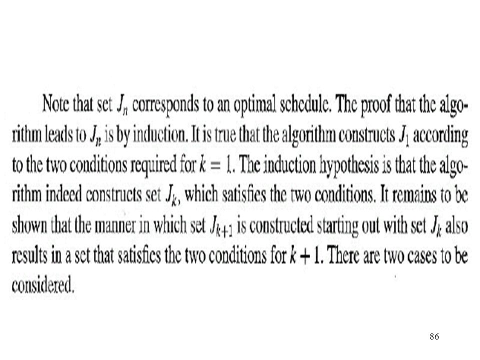
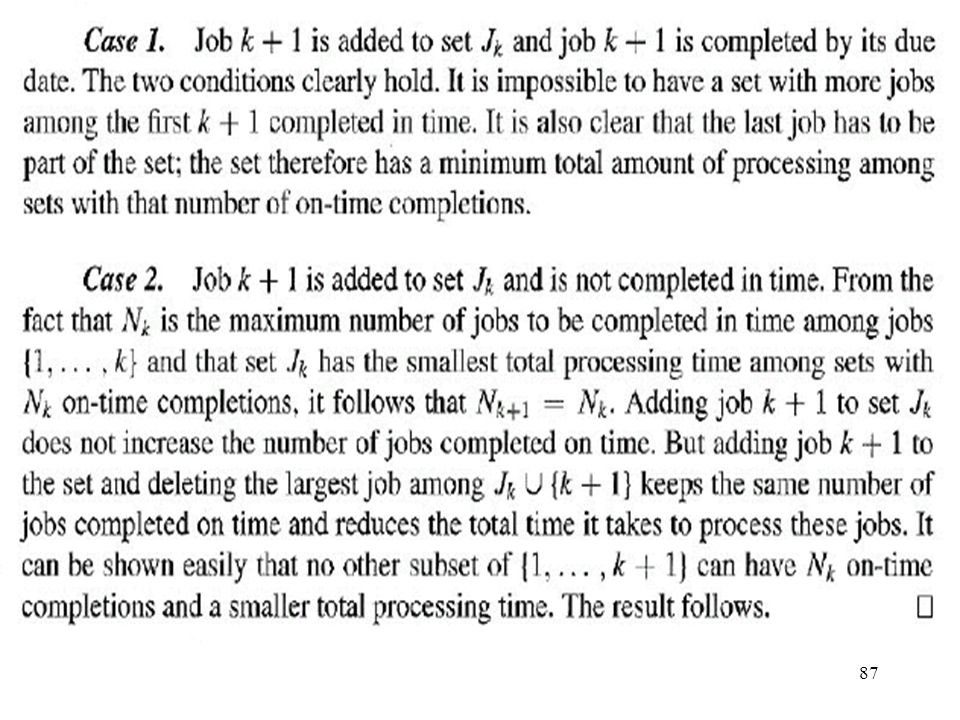
85
Theorem 3.3.2. Algorithm 3.3.1 yields an optimal schedule for 1 || Uj

88
j*=1 J = {1} , Jd = , JC = {2, 3, 4, 5}, t=7 < 9 = d1
Example J = , Jd = , JC = {1,...,5} j*=1 J = {1} , Jd = , JC = {2, 3, 4, 5}, t=7 < 9 = d1 7 1 j*=2 J = {1, 2} , Jd = , JC = {3, 4, 5}, t=15 < 17 = d2 7 1 2 15 j*=3 J = {1, 2, 3} , Jd = , JC = {4, 5}, t=19 > 18 = d3 k*=2 J = {1, 3} , Jd = {2}, t=11 7 1 2 15 3 19

89
j*=4 J = {1, 3, 4} , Jd = {2}, JC = {5}, t=17 < 19 = d4
15 4 17 j*=5 J = {1, 3, 4, 5} , Jd = {2}, JC = , t=23 > 21 = d5 k*=1 J = {3, 4, 5} , Jd = {2, 1}, t=16 < 21 = d5 7 1 3 15 4 17 5 23 optimal schedule 3, 4, 5, 1, 2 Uj = 2

90
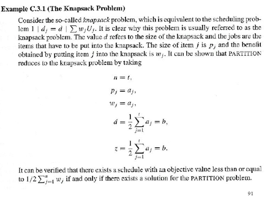
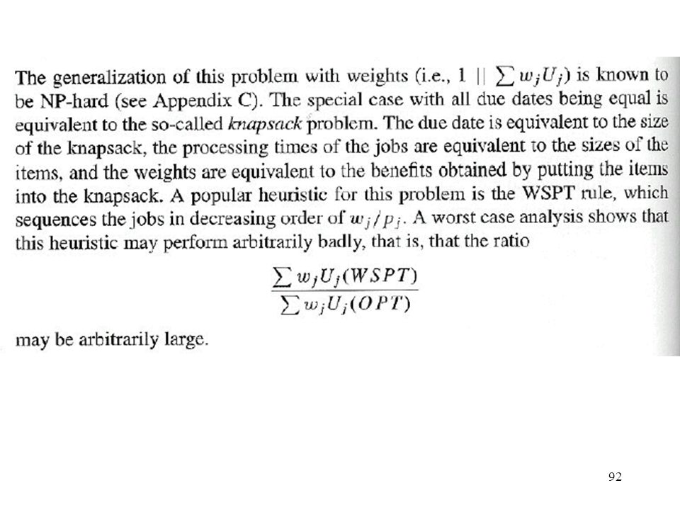
Although 1 || Uj can be done in O(n log(n)) , 1 || wjUj is NP hard.
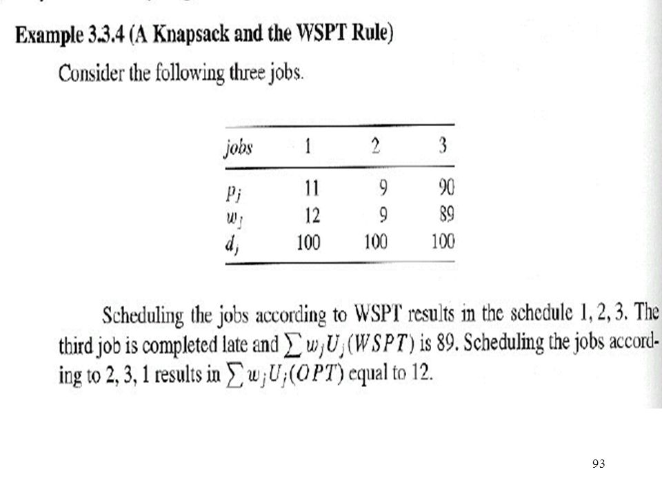
The problem 1 || wjUj is equivalent to the so-called Knapsack Problem.

94
The Total Tardiness 1 || Tj is NP hard
Lemma If and then there exists an optimal sequence in which job j is scheduled before job k. Proof Sum of tardiness of job j and k :

95
Sum of tardiness of job j and k :
In the following, we are going to show that Let Thus, we are going to show that

96
Case I : Three cases Case II : Case III : Case I : If

97
Case II : If Since so thus i.e.

98
Case III : It can be easily checked that

99
Moreover, the worst case (most negative) for
Since the most negative case for would be when

100
i.e.

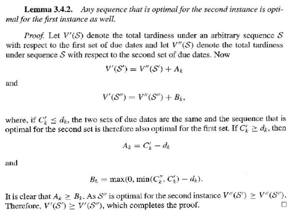
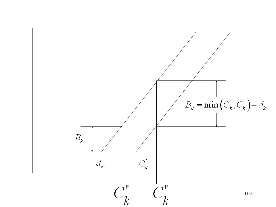
103
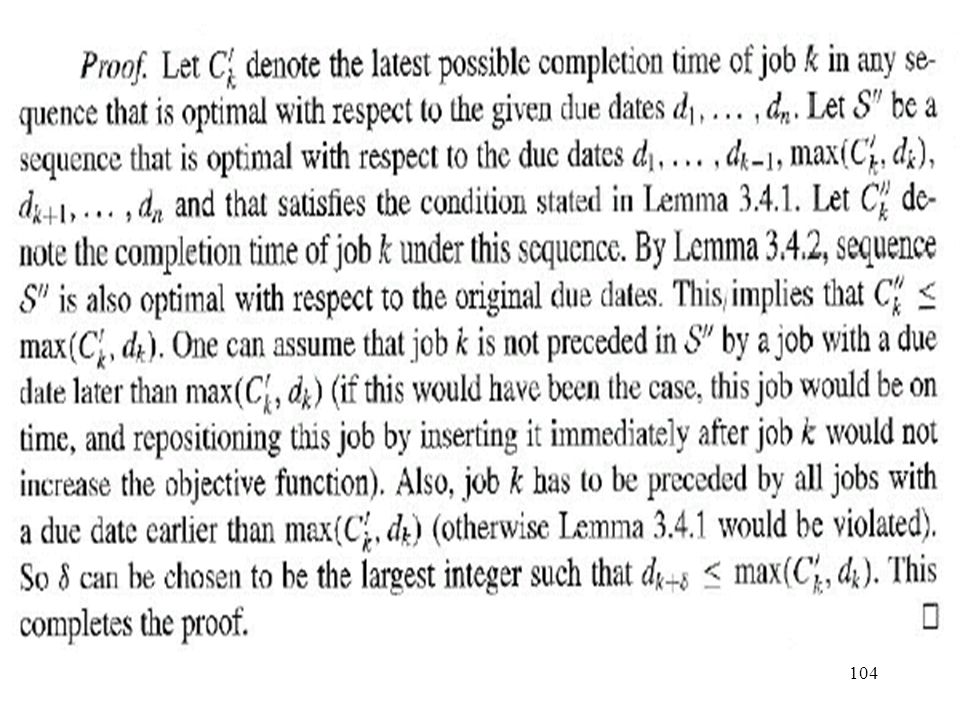
Lemma.3.4.3. There exists an integer , 0 n-k such that there is
an optimal schedule S in which job k is preceded by jobs j k + and followed by jobs j > k + . completion time of job k {1, ... ,k-1, k+1, ..., k+ } any order {k++1, ..., n} k

105
PRINCIPLE OF OPTIMALITY
Assertion: If abe is the optimal path from a to e, then be is the optimal path from b to e. Proof: Suppose it is not. Then there is another path (note that existence is assumed here) bce which is optimal from b to e, i.e. Jbce > Jbe but then Jabe = Jab+Jbe< Jab+ Jbce= Jabce This contradicts the hypothesis that abe is the optimal path from a to e. Jbe Jab b Jbce e
 bce which. is optimal from b to e, i.e. Jbce > Jbe. but then. Jabe = Jab+Jbe< Jab+ Jbce= Jabce. This contradicts the hypothesis that abe is the. optimal path from a to e. Jbe. Jab. b. Jbce. e.")
106
A Dynamic Programming Example
Stagecoach Problem Costs:

107
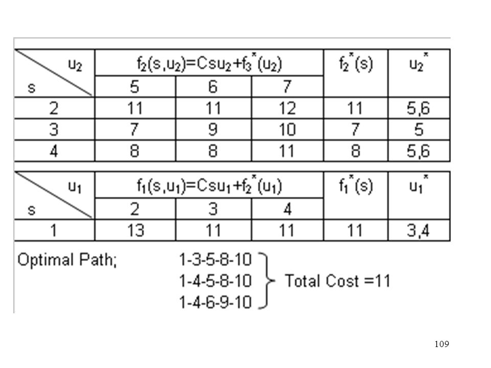
Solution: Let 1-u1-u2-u3-10 be the optimal path. Let fn(s,un) be the minimal cost path given that current state is s and the decision taken is un . fn*(s) = min f (s,un) = min {cost(s, un) +fn+1*(un) } un un This is the Recursion Equation of D.P. It can be solved by a backward procedure – which starts at the terminal stage and stops at the initial stage.
 = min f (s,un) = min {cost(s, un) +fn+1*(un) } un un. This is the Recursion Equation of D.P. It can be. solved by a backward procedure – which starts at. the terminal stage and stops at the initial stage.")
108
Note: 1-2-6-9-10 with cost=13 is a greedy path that
minimizes cost at each stage. This may not be minimal cost solution, however, e.g is cheaper overall than

110
PRINCIPLE OF OPTIMALITY, Bellman 1956.
An optimal policy has the property that whatever the initial state and the initial decision are, the remaining decisions must constitute an optimal policy with regard to the state resulting from the first decision. Algorithm Dynamic programming procedure: recursively the optimal solution for some job set J starting at time t is determined from the optimal solutions to subproblems defined by job subsets of S*S with start times t*t . J(j, l, k) contains all the jobs in a set {j, j+1, ... , l} with processing time pk V( J(j, l, k) , t) total tardiness of the subset under an optimal sequence if this subset starts at time t
 contains all the jobs in a set {j, j+1, ... , l} with processing time pk. V( J(j, l, k) , t) total tardiness of the subset under an optimal sequence. if this subset starts at time t.")
111
Initial conditions: V(, t) = 0 V( { j }, t ) = max (0, t + pj - dj) Recursive conditions: where k' is such that pk' = max ( pj' | j' J(j, l, k) ) Optimal value function is obtained for V( { 1,...,n }, 0 )
 ) Optimal value function is obtained for. V( { 1,...,n }, 0 )")
112
Example k'=3, 0 2 dk' = d3 = 266 C3(0) - d3 = 81, C3(1) - d3 = 164, C3(2) - d3 = 294, = 81, =347 =164, =430 =294, =560

113
V( J(1, 3, 3) , 0) = , 2 C1 = 121 C2 = =200 T1 =max(0, C1 – d1) =max(0, )=0 T2 =max(0, C2 - d2) =max(0, )=0 T1+ T2 = 0 2, 1 C2 = 79 C1 = =200 =max(0, )=0 =max(0, )=0 T2+ T1 = 0
 =max(0, )=0. T1+ T2 = 0. 2, 1 C2 = 79. C1 = =200. =max(0, )=0. =max(0, )=0. T2+ T1 = 0.")
114
V( J(4, 5, 3) , 347) 4, 5 T4 = max(0, ) = 94 T5 = max(0, )=223 T4 + T4 = 317 5, 4 T5 = max(0, )= 140 T4 = max(0, )=224 T5+ T4 = 364 V( J(1, 4, 3) , 0)=0 achieved with the sequence 1, 2, 4 and 2, 1, 4 V( J(5, 5, 3) , 430)=223 V( J(1, 5, 3) , 0)=76 achieved with the sequence 1, 2, 4, 5 and 2, 1, 4, 5 V( , 560)=0 optimal sequences: 1, 2, 4, 5, 3 and 2, 1, 4, 5, 3
= 140. T4 = max(0, )=224. T5+ T4 = 364. V( J(1, 4, 3) , 0)=0 achieved with the sequence 1, 2, 4 and 2, 1, 4. V( J(5, 5, 3) , 430)=223. V( J(1, 5, 3) , 0)=76 achieved with the sequence 1, 2, 4, 5 and 2, 1, 4, 5. V( , 560)=0. optimal sequences: 1, 2, 4, 5, 3 and. 2, 1, 4, 5, 3.")
115
Summary 1 || Uj forward algorithm 1 || wjUj is NP hard
1 || Tj is NP hard, pseudo-polynomial algorithm based on dynamic programming

116
The Total Weighted Tardiness
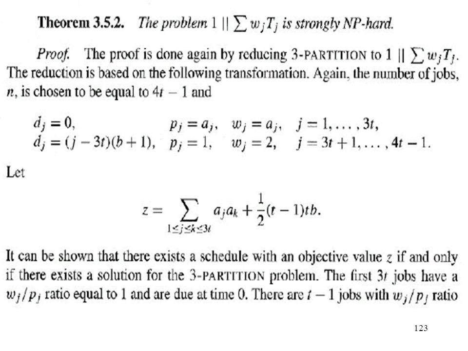
1 || wjTj is strongly NP hard Lemma If , and then there exists an optimal sequence in which job j is scheduled before job k. Proof Sum of weighted tardiness of job j and k :

117
Sum of weighted tardiness of job j and k :
In the following, we are going to show that Let Thus, we are going to show that

118
Case I : Three cases Case II : Case III : Case I : If

119
Case II : If Since so thus i.e. so

120
Case III : It can be easily checked that

121
Moreover, the worst case (most negative) for
Since the most negative case for would be when

122
i.e. Moreover so

125
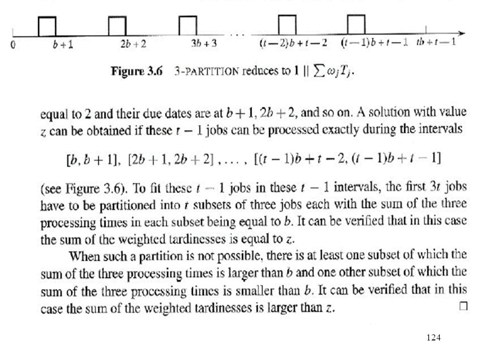
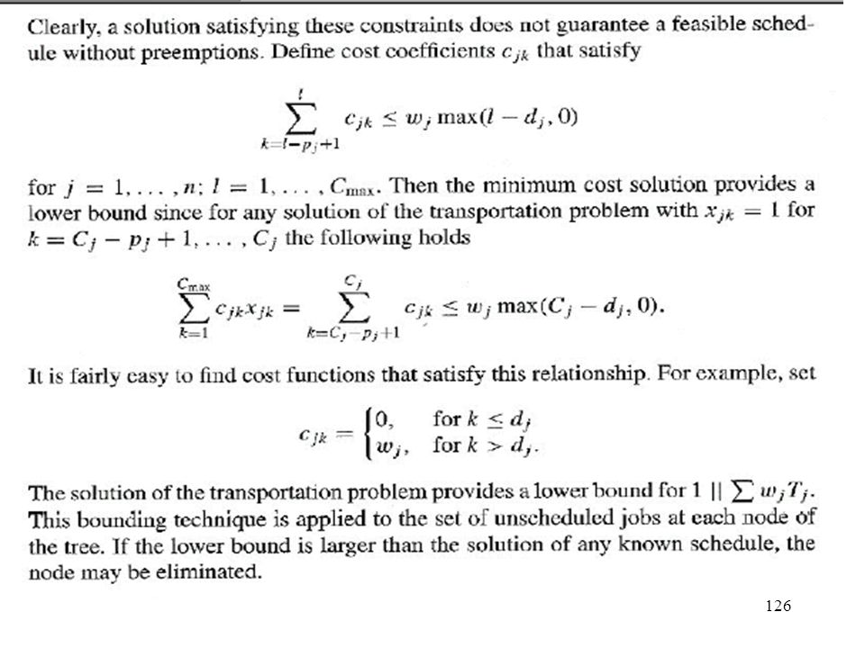
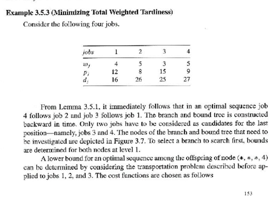
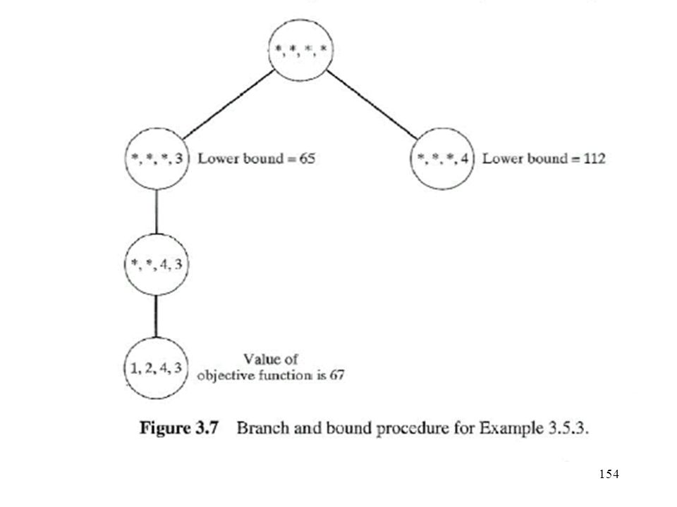
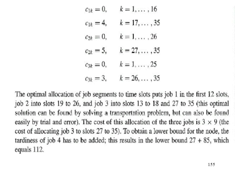
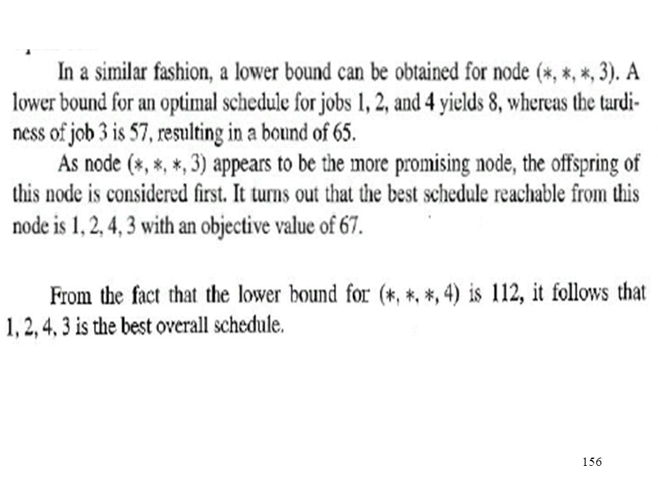
Usually, branch and bound approach is used for 1 || wjTj.
How do we find the bound ? There are many different bounding techniques. Relaxation of the problem to a Transportation problem. Each job j with (integer) processing time pj is divided into pj jobs, each with unit processing time. The decision variables xjk is 1 if one unit of job j is processed during the time interval [k-1,k] and 0 otherwise. These decision variables must satisfy
 processing time pj is divided into pj jobs, each with unit processing time. The decision variables xjk is 1 if one unit of job j is processed during. the time interval [k-1,k] and 0 otherwise. These decision variables must. satisfy.")
127
Transportation Problem
The transportation problem seeks to minimize the total shipping costs of transporting goods from m origins (each with a supply si) to n destinations (each with a demand dj), when the unit shipping cost from an origin, i, to a destination, j, is cij. AMA522 Scheduling
 to n destinations (each with a demand dj), when the unit shipping cost from an origin, i, to a destination, j, is cij. AMA522 Scheduling.")
128
Transportation Problem
1 Network Representation d1 c11 1 c12 s1 c13 2 d2 c21 c22 2 s2 c23 3 d3 SOURCES DESTINATIONS AMA522 Scheduling

129
Transportation Problem
LP Formulation The linear programming formulation in terms of the amounts shipped from the origins to the destinations, xij, can be written as: Min SScijxij i j s.t. Sxij < si for each origin i j Sxij = dj for each destination j i xij > 0 for all i and j AMA522 Scheduling

130
Transportation Problem
LP Formulation Special Cases The following special-case modifications to the linear programming formulation can be made: Minimum shipping guarantees from i to j: xij > Lij Maximum route capacity from i to j: xij < Lij Unacceptable routes: delete the variable AMA522 Scheduling

131
Example: BBC Building Brick Company (BBC) has orders for 80 tons of bricks at three suburban locations as follows: Northwood tons, Westwood tons, and Eastwood tons. BBC has two plants, each of which can produce 50 tons per week. How should end of week shipments be made to fill the above orders given the following delivery cost per ton: Northwood Westwood Eastwood Plant Plant AMA522 Scheduling
 has orders for 80 tons of bricks at three suburban locations as follows: Northwood tons, Westwood tons, and Eastwood tons. BBC has two plants, each of which can produce 50 tons per week. How should end of week shipments be made to fill the above orders given the following delivery cost per ton: Northwood Westwood Eastwood. Plant Plant AMA522 Scheduling.")
132
xij = amount shipped from plant i to suburb j
LP Formulation Decision Variables Defined xij = amount shipped from plant i to suburb j where i = 1 (Plant 1) and 2 (Plant 2) j = 1 (Northwood), 2 (Westwood), and 3 (Eastwood) AMA522 Scheduling
 and 2 (Plant 2) j = 1 (Northwood), 2 (Westwood), and. 3 (Eastwood) AMA522 Scheduling.")
133
s.t. x11 + x12 + x13 < 50 (Plant 1 capacity)
LP Formulation Objective Function Minimize total shipping cost per week: Min 24x x x x x x23 Constraints s.t. x11 + x12 + x13 < 50 (Plant 1 capacity) x21 + x22 + x23 < 50 (Plant 2 capacity) x11 + x21 = 25 (Northwood demand) x12 + x22 = 45 (Westwood demand) x13 + x23 = 10 (Eastwood demand) all xij > (Non-negativity) AMA522 Scheduling
 x21 + x22 + x23 < 50 (Plant 2 capacity) x11 + x21 = 25 (Northwood demand) x12 + x22 = 45 (Westwood demand) x13 + x23 = 10 (Eastwood demand) all xij > 0 (Non-negativity) AMA522 Scheduling.")
134
Partial Spreadsheet Showing Problem Data
AMA522 Scheduling

135
Partial Spreadsheet Showing Optimal Solution
AMA522 Scheduling

136
Optimal Solution From To Amount Cost Plant 1 Northwood 5 120
Plant 1 Westwood ,350 Plant 2 Northwood Plant 2 Eastwood Total Cost = $2,490 AMA522 Scheduling

137
Linear programming (LP) model
Matrix form: objective function constraints variable restrictions where: x, c: n-vector A: m,n-matrix b: m-vector

138
Linear programming example
or:

139
Linear programming example: graphical solution (2D)
6 5 4 3 2 1 1 2 3 4 5 6 solution space x1

140
Linear programming (cont.)
Solution techniques: (dual) simplex method interior point methods (e.g. Karmarkar algorithm) Commercial solvers, for example: CPLEX (ILOG) XPRESS-MP (Dash optimization) OSL (IBM) Modeling software, for example: AIMMS AMPL
 simplex method. interior point methods (e.g. Karmarkar algorithm) Commercial solvers, for example: CPLEX (ILOG) XPRESS-MP (Dash optimization) OSL (IBM) Modeling software, for example: AIMMS. AMPL.")
141
Integer programming (IP) models
Integer variable restriction IP: integer variables only MIP: part integer, part non-integer variables BIP: binary (0-1) variables General IP-formulation: Complex solution space
 variables. General IP-formulation: Complex solution space.")
142
Integer programming example: graphical solution (2D)
6 5 4 3 2 1 2 optimal solutions! 1 2 3 4 5 6 x1

143
Total unimodularity property for integer programming models
Suppose that all coefficients are integer in the model: i.e. Example: transportation problem if A has the total unimodularity property (i.e. every square submatrix has determinant 0,1,-1) Þ there is an optimal integer solution x* & the simplex method will find such a solution
 Þ there is an optimal integer solution x* & the simplex method will find such a solution.")
144
Integer programming tricks
PROBLEM: x = 0 or x k use binary indicator variable y= restrictions:

145
Integer programming tricks (2)
PROBLEM: fixed costs: if xi>0 then costs C(xi) use indicator variable yi= restrictions :
 use indicator variable yi= restrictions :")
146
(Integer) programming tricks (3)
Hard vs. soft restrictions hard restriction: must hold, otherwise unfeasibility for example: soft restriction: may be violated, with a penalty

147
(Integer) programming tricks (4)
Absolute values: solution: goal variation

148
Integer programming tricks (5)
Conjunctive/disjunctive programming - conjunctive set of constraints: must all be satisfied - disjunctive set of constraints: at least one must be satisfied example :

149
nonpreemptive single machine, total weighted completion time
IP example nonpreemptive single machine, total weighted completion time model definition: objective function: minimize weighted completion time:

150
IP example (cont.) Restriction: all jobs must be completed once:
Restriction: only one job per time t: if job j is in process during t, it must be completed somewhere during [t,t+pj]

151
IP example (cont.) Complete IP-model: nCmax integer variables
 Complete IP-model: nCmax integer variables")
152
Additional restriction: precedence constraints
IP example (cont.) Additional restriction: precedence constraints Model definition: SUCC(j) = successors of job j job j must be completed before all jobs in SUCC(j):
 Additional restriction: precedence constraints. Model definition: SUCC(j) = successors of job j. job j must be completed before all jobs in SUCC(j):")
Similar presentations


 Marc E Posner (Ohio State University) Chris N Potts (University of Southampton)>")


>")


