1. Fisheye Camera Calibration Arunkumar Byravan & Shai Revzen University of Pennsylvania

2. Camera Calibration is mainly concerned with finding the parameters intrinsic to the camera that affect the imaging process, namely: The focal length of the lens The principal point of the lens Scaling & Skew factors The lens projection/distortion function These parameters are important and necessary for various Structure From Motion, 3D reconstruction and other applications where the relation between world points and camera pixels are needed.

3. The need to calibrate a fisheye camera in order to solve the odometry problem. Initially tried out a few existing toolboxes, namely the Camera Calibration Toolbox for Matlab & Omnidirectional camera calibration Toolbox Results were not good enough which led us to work on our own calibration method.

4. Fisheye lenses are those which have a very high Field Of View ( >= 150 degrees). Fisheye lenses achieve extremely wide angles of view by forgoing a rectilinear image, opting instead for a special mapping (for example: equisolid angle), which gives images a characteristic convex appearance. Due to the high degree of distortion in the image, such images are difficult to process using conventional techniques which are meant for perspective cameras. Our camera is fitted with a 190 degree FOV lens from Omnitech Robotics.

5. An Image from the camera

6. Lots of work in Photogrammetry & more recently in the Computer Vision community. Roughly two categories: Photogrammetric calibration Uses a Calibration object. Self Calibration Uses the motion of camera in a static scene. Correspondences between 3 images are enough to recover the parameters. Other techniques exist, which use orthogonal vanishing points or pure rotation of cameras for calibration.

8. Slide courtesy of Prof. Ramani Duraiswami, Dept. of Computer Science, UMCP.

9. Slide courtesy of Prof. Ramani Duraiswami, Dept. of Computer Science, UMCP.

10. Slide courtesy of Prof. Ramani Duraiswami, Dept. of Computer Science, UMCP.

11. Slide courtesy of Prof. Ramani Duraiswami, Dept. of Computer Science, UMCP.

12. Slide courtesy of Prof. Ramani Duraiswami, Dept. of Computer Science, UMCP.

13. Slide courtesy of Prof. Ramani Duraiswami, Dept. of Computer Science, UMCP.

14. Slide courtesy of Prof. Ramani Duraiswami, Dept. of Computer Science, UMCP.

15. Slide courtesy of Prof. Ramani Duraiswami, Dept. of Computer Science, UMCP.

16.  In all the above slides, the assumption was that there is no lens distortion.  In the presence of distortion, the actual pixel location will be different from [x pix y pix ] T  Two main distortion effects:  Radial Distortion : Barrel, Pincushion distortion  Tangential Distortion : due to “Decentering”  Widely used “Plumb Bob” distortion model was introduced by Brown in 1966.

17.  [u, v] are final pixel values after distortion.  K is the Intrinsic camera matrix.

18.  Print a calibration pattern (checkerboard) & attach it to a planar surface.  Take a few pictures of the pattern under different orientations by moving the camera or the pattern.  Detect the corners of the checkerboard.  Now we have a set of world points whose image correspondences are known.  Get an initial estimate of the Rotation & Translation ( & maybe intrinsic parameters) between the world frame& camera frame using the DLT algorithm(many other ways to do this).

19.  Minimise the reprojection error using some non- linear minimisation technique to get better estimates of parameters.  Lots of ways to actually compute the parameters.  Huge amount of literature using different techniques.

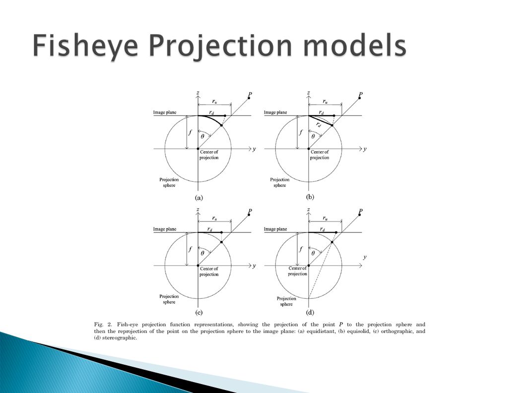
21.  The fisheye lens can be modeled as a “projection function” that takes a point on the unit sphere onto a point on the image plane.  In spherical coordinates, this is a function of the elevation angle (θ) & maybe the angle in the plane (φ).  It is of the form, where r = radial distance of a point from the image centre. g = lens projection function.

22.  Examples of general lens projection functions which conform to different models are: ◦ Equidistant projection model: ◦ Equisolid projection model : ◦ Stereographic projection model: ◦ Orthographic projection model: Where f = focal length of the camera.

24.  In our current calibration, we have modeled this “projection function” as a polynomial function of θ. where the A i ’s are constants to be estimated & “φ” is the angle in the image plane.  Initially, we had tried to use the general fisheye models (shown before) as a basis for “g”, but the accuracy achieved was not good enough.

25.  Initially, we have a set of checkerboard images.  After corner extraction, we have a set of points in the image which have corresponding world points.  We initially assume that, g(θ,φ) = f*θ  Also, assume the principal point [u 0,v 0 ] T to be at the centre of the image.

26.  “m” is a pixel.  “m 0 ” is the principal point.  f i is an initial estimate of the focal length.  is a point in the camera reference frame.

27.  M is a point in the world reference frame.  and M are related by a rotation & translation.  This is found using the procedure in [1].

28.  With the initial estimates of R & t, we now minimise the reprojection error to find the suitable parameters.

29. where [x, y] is the actual image point. By minimising this, we can get the parameters that best suit the camera & lens.

30.  Initial testing with a set of 5 images shows good results.  Reprojection error in the range of 0.3 – 0.5 pixels.  Minimization is done just a single time and the dimension of the feature vector is very large.  Also, and s=0 for this trial (no skew & pixels are assumed to be square).

31.  Analyzing the results show that most of the error is due to poor corner detection.  Better corner detection may increase accuracy.  Lots of optimizations can be done to improve speed & performance.

32.  Repeating the whole procedure more than once may yield better results.  Can be made more robust by use of better geometric constraints?  Can be theoretically extended to perspective cameras as well.

33. [1] Richard J. Hanson And Michael J. Norris, “Analysis Of Measurements Based On The Singular Value Decomposition,” Siam J. Sci. Stat. Comput., Vol. 2, No. 3, September 1981 [2] D. C. Brown, “Decentering distortion of lenses,” Photograph. Eng. 32, 444–462 (1966). [3] R. Tsai, “A versatile camera calibration technique for high accuracy 3D machine vision metrology using off-the-shelf TV cameras and lenses,” IEEE Trans. Robot. Automat. 3, 323–344 (1987). [4] Z. Zhang, “A flexible new technique for camera calibration,” IEEE Trans. Pattern Anal. Mach. Intell. 22, 1330–1334 (2000). [5] Camera Calibration Toolbox for Matlab, http://www.vision.caltech.edu/bouguetj/calib_doc/index.html http://www.vision.caltech.edu/bouguetj/calib_doc/index.html [6] Lecture Notes from CMSC 828D: Fundamentals of Computer Vision http://www.umiacs.umd.edu/~ramani/ [7] Ciarán Hughes, Patrick Denny, Edward Jones, and Martin Glavin, Accuracy of fish-eye lens models, Applied Optics / Vol. 49, No. 17 / 10 June 2010