Download presentation
Presentation is loading. Please wait.

1
William Ahue University of Wisconsin – Madison Dept. of Atmospheric and Oceanic Sciences Department Seminar 28 April 2010 Advisor: Prof. Ankur Desai

2
Motivation and Background Why study carbon dioxide? Why study boundary layers in mountainous terrain? What is ACME? Data and Methods Boundary Layer Budget Method Determination of Boundary Layer Heights Profile Matching Results Summary and Future Work

3
All life begins and ends with carbon NASA/NASA Earth Science Enterprise

4
NOAA ESRL, 2010 Biosphere

6
Onset of Spring Summer Drought Summer Monsoon Courtesy of R. Monson, CU-Boulder

7
Forest ecosystem is an important carbon sink (Schmil et al., 2002) Ongoing stresses add to the uncertainty about future carbon uptake (Raffa et al., 2008) CO 2 land-atmosphere exchange is poorly constrained in global models (Schmil et al., 2002) Data rich location http://www.destination360.com
 Ongoing stresses add to the uncertainty about future carbon uptake (Raffa et al., 2008) CO 2 land-atmosphere exchange is poorly constrained in global models (Schmil et al., 2002) Data rich location")
8
AP Photo/Peter M. Fredin Photo Credit: Shawn Martini

9
Interactions between terrain and overlying atmosphere lead to complex flows Determines how carbon dioxide is mixed vertically and its exchange with the free troposphere Whiteman, 2000

10
Field experiment that flew paired morning upwind and afternoon downwind profiles to measure carbon in the Central Rocky Mountains Collected airborne measurements of CO, CO 2, O 2 and H 2 O as well as other atmospheric variables Over 60 hours of flight time from May to August University of Wyoming’s King Air Aircraft First conducted in 2004 (Sun et al., 2010) Methods were improved for 2007
 Methods were improved for 2007")
11
UPWIND DOWNWIND

12
Experiment was conducted in the Central Rocky Mountains Complex terrain with various mesoscale flows Used multiple parallel profiles http://roadtripusa.net

13
Complex terrain imparted flux variations Multiple parallel profile approach needed Vertical shear was large Valley cold pools vented later than expected Shifted times of flights

14
What is the magnitude of carbon uptake in the Central Rocky Mountains? How do flux estimates from the boundary layer budget (BLB) method compare with CarbonTracker and Niwot Ridge? What is the uncertainty of boundary layer heights in the region?
 method compare with CarbonTracker and Niwot Ridge. What is the uncertainty of boundary layer heights in the region .")
15
Motivation and Background Why study carbon dioxide? Why study boundary layers in mountainous terrain? What is ACME? Data and Methods Boundary Layer Budget Method Determination of Boundary Layer Heights Profile Matching Results Summary and Future Work

16
Top-Down Based on inversions of atmospheric concentrations Particle transport models, running in the back trajectory mode, are used to obtain influence functions Bottom- up Local processes are scaled up in time and space from the site level Limited by the accuracy and spatial footprint of the measurements UN FAO, 2010

17
Why not use an inverse model?? It is HARD!!! Global inverse models provide too coarse a resolution Regional inverse models require good inflow fluxes and accurate assimilation methods Also have to account for spatial heterogeneity and local processes

18
Column averaged variations are not affected by variations in boundary layer height Issues with Method Ability to track air masses from one region to another Requires accurate estimates of boundary layer height

19
The convective boundary layer is a vertically confined column of air (Stull, 1988; Garrat, 1990) It incorporates overlaying air into it as it grows Resolves issues with vertical entrainment Bulk properties of the column are independent of small scale heterogeneities (Stull, 1988; Garrat, 1990) Natural integrator of surface fluxes over complex terrain Simulations with idealized initial conditions using RAMS show PBL max to be a good proxy when compared with observations (DeWekker, in prep)
 It incorporates overlaying air into it as it grows Resolves issues with vertical entrainment Bulk properties of the column are independent of small scale heterogeneities (Stull, 1988; Garrat, 1990) Natural integrator of surface fluxes over complex terrain Simulations with idealized initial conditions using RAMS show PBL max to be a good proxy when compared with observations (DeWekker, in prep)")
20
Three different estimates of boundary layer heights were obtained North American Regional Reanalysis Model (NARR) TKE based method Parcel Method Visual inspections of vertical profiles of Virtual Potential Temperature and Water Vapor Mixing Ratio Bulk Richardson Number Ri c = 0.25 (Pleim and Xiu, 1995)
 TKE based method Parcel Method Visual inspections of vertical profiles of Virtual Potential Temperature and Water Vapor Mixing Ratio Bulk Richardson Number Ri c = 0.25 (Pleim and Xiu, 1995)")
21
Particle dispersion results from 5 receptors and various forecast models were used to determine likely source locations Using an least squares estimate, distance from the centroid of the released particles to the flight path were determined This distance was used to determine which receptor the air sampled in the morning belonged to (Source)
")
22
Afternoon flight flew diving spirals around each receptor location (Sink) Air sampled from the flight profile for each receptor source and sink were used to determine the receptor’s flux
 Air sampled from the flight profile for each receptor source and sink were used to determine the receptor’s flux")
23
NEE from Niwot Ridge AmeriFlux Tower NEE from 2008 release of CarbonTracker (NOAA ESRL) Airborne Observations from seven flight days NARR Boundary Layer Heights (NOAA NCEP) Photo Credit: Vanda Grubisic, DRI
 Airborne Observations from seven flight days NARR Boundary Layer Heights (NOAA NCEP) Photo Credit: Vanda Grubisic, DRI")
24
Regional Atmospheric Modeling System (RAMS) Version 6.0 06 UTC 21 June 07 to 00 UTC 22 June 07 Domain centered at 40N, 106.5W 1.5 km Resolution Hybrid Particle and Concentration Transport Model (HYPACT) Lagrangian Particle Dispersion Model 5 source locations from the morning flight profile from 21 June 07 1000 particles were released at 15 UTC 21 June 07 Source located 100 m AGL
 Version UTC 21 June 07 to 00 UTC 22 June 07 Domain centered at 40N, 106.5W 1.5 km Resolution Hybrid Particle and Concentration Transport Model (HYPACT) Lagrangian Particle Dispersion Model 5 source locations from the morning flight profile from 21 June particles were released at 15 UTC 21 June 07 Source located 100 m AGL")
25
Motivation and Background Why study carbon dioxide? Why study boundary layers in mountainous terrain? What is ACME? Data and Methods Boundary Layer Budget Method Determination of Boundary Layer Heights Profile Matching Results Summary and Future Work

26
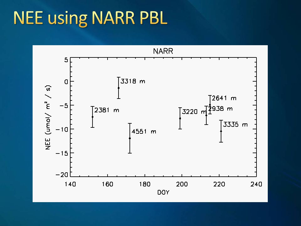
Evaluation of RAMS and HYPACT Does the Experimental Design Work? Initial Boundary Layer Budget Fluxes using NARR PBL Estimation and Comparison of Boundary Layer Heights Boundary Layer Budget Fluxes Revisited Receptor and Receptor Averaged Fluxes

27
Niwot RidgeStorm Peak Lab Observations Model

29
Evaluation of RAMS and HYPACT Does the Experimental Design Work? Initial Boundary Layer Budget Fluxes using NARR PBL Estimation and Comparison of Boundary Layer Heights Boundary Layer Budget Fluxes Revisited Receptor and Receptor Averaged Fluxes

31
Niwot Ridge CarbonTracker BLB

32
Evaluation of RAMS and HYPACT Does the Experimental Design Work? Initial Boundary Layer Budget Fluxes using NARR PBL Estimation and Comparison of Boundary Layer Heights Boundary Layer Budget Fluxes Revisited Receptor and Receptor Averaged Fluxes

33
Morning Afternoon PBL Max = 3648

35
Evaluation of RAMS and HYPACT Does the Experimental Design Work? Initial Boundary Layer Budget Fluxes using NARR PBL Estimation and Comparison of Boundary Layer Heights Boundary Layer Budget Fluxes Revisited Receptor and Receptor Averaged Fluxes

36
Niwot Ridge CarbonTracker BLB

38
Evaluation of RAMS and HYPACT Does the Experimental Design Work? Initial Boundary Layer Budget Fluxes using NARR PBL Estimation and Comparison of Boundary Layer Heights Boundary Layer Budget Fluxes Revisited Receptor and Receptor Averaged Fluxes

39
Niwot Ridge CarbonTracker BLB

40
Niwot Ridge CarbonTracker BLB

41
Niwot Ridge CarbonTracker BLB

42
Niwot Ridge CarbonTracker BLB

44
Motivation and Background Why study carbon dioxide? Why study boundary layers in mountainous terrain? What is ACME? Data and Methods Boundary Layer Budget Method Determination of Boundary Layer Heights Profile Matching Results Summary and Future Work

45
Meteorological observations from Niwot Ridge and Storm Peak Lab show general agreement with RAMS Difference are most likely caused by local processes not capture by the model HYPACT results validates experimental design Able to chase air using morning downwind / afternoon up flight profiles

46
CarbonTracker shows less uptake in mid- summer when compared to Niwot Ridge and airborne observations Initial BLB fluxes shows broad agreement among the three methods Accurate estimates of boundary layer growth required to further narrow the uncertainty of carbon fluxes in complex terrain General agreement among all estimates of PBL

47
Receptor fluxes show broad agreement when compared with Niwot Ridge and CarbonTracker Some receptor fluxes show larger uptake How do you compare fluxes that vary in scale, time and method of calculation? With the exception of two flight day, receptor averaged fluxes compare well with fluxes calculated using the entire flight profile Spatial and temporal averages of CarbonTracker fluxes over the domain show an inverse relationship when compared with airborne observations

48
Run RAMS simulations for remaining flight days Using RAMS output, Run HYPACT Release particles along entire morning upwind flight profile to determine its influence on the afternoon downwind flight profile Assimilate airborne observations into a regional inverse model Top-down Approach Compare BLB flux estimates with an ecosystem model (i.e. SIPNET) Bottom-up Approach
 Bottom-up Approach.")
49
My Advisor: Prof. Ankur Desai M.S. Thesis Readers: Prof. Galen McKinley and Prof. Dave Turner Rest of the ACME Collaborators Stephan DeWekker (UVa) Teresa Campos (NCAR) Fellow Grad Students AOS Faculty and Staff Funding Sources: DoD SMART Scholarship NSF and NOAA UW Graduate School
 Teresa Campos (NCAR) Fellow Grad Students AOS Faculty and Staff Funding Sources: DoD SMART Scholarship NSF and NOAA UW Graduate School.")
Similar presentations


 over Mesoscale Surface Heterogeneity 25 June 2009 Song-Lak Kang Research Review.>")


 for the June, July, August and September 2000 Simulation: RAMS v4.3 with two nested grids (Δx=100km and.>")

