1. ANALYSIS OF VARIANCE  Gerry Quinn & Mick Keough, 1998 Do not copy or distribute without permission of authors. One factor

2. Barnacle recruitment Effects of 4 surface types on barnacle recruitment on rocky shore Surface type is independent variable: –alga sp.1, alga sp.2, bare rock, scraped rock Independent variable: –categorical with 2 or more levels –factor –levels termed groups (“treatments”)

3. Five replicate plots for each surface type Dependent (response) variable: –number barnacles after 4 weeks etc. Bare Alg 2 Scraped Alg 1 Scraped

4. 2724912 1933138 18271715 23261420 25322211 Treatment group: Alga sp.1Alga sp.2BareScraped Data Number of barnacles per plot

5. ANOVA vs regression One factor ANOVA: –1 continuous dependent variable and 1 categorical independent variable (factor) Compare with regression: –1 continuous dependent variable and 1 continuous independent variable

6. Aims Measure relative contribution of different sources of variation (factors or combination of factors) to total variation in dependent variable Test hypotheses about group (treatment) population means for dependent variable

7. Terminology Factor (independent variable): –usually designated factor A –number of levels/groups/treatments = a Number of replicates within each group –n–n Each observation: –y–y

8. Data layout Factor level (group)12…i Replicatesy 11 y 21...y i1 y 1j y 2j...y ij............ y 1n y 2n...y in Population means  1  2  i Sample means y 1 y 2 y i Grand mean y estimates 

9. Alg sp1Alg sp2BareScraped y 11 =27y 21 =24y 31 = 9y 41 =12 y 12 =19y 22 =33y 32 =13y 42 = 8 y 13 =18y 23 =27y 33 =17y 43 =15 y 14 =23y 24 =26y 34 =14y 44 =20 y 15 =25y 25 =32y 35 =22y 45 =11 Means:22.428.415.013.2 Overall mean: 19.75

10. Linear model for 1 factor ANOVA The linear model for 1 factor ANOVA: y ij =  +  i +  ij where  = overall population mean  i = effect of ith treatment or group (  -  i )  ij = random or unexplained error (i.e. variation not explained by treatment effects)

11. Compare with regression model y i =  0 +  1 x 1 +  i intercept is replaced by  slope is replaced by  i (treatment effect): –independent variable is categorical rather than continuous –still measures “effect” of independent variable

12. Types of factor Fixed factor: –all levels or groups of interest are used in study –conclusions are restricted to those groups Random factor: –random sample of all groups of interest are used in study –conclusions extrapolate to all possible groups

13. Null hypothesis Ho:  1 =  2 =  i =  No difference between population group (treatment) means Mean number of barnacle recruits is same on four substrata

14. H O - fixed factor Treatment or group effects:  1 = (  1 -  ),  2 = (  2 -  ),  i = (   -  ) where  i = the effect of group or treatment i H O :  1 =  2 =  i = 0 No group (treatment) effects No effect of any surface type on barnacle recruitment

15. H O - random factor H O :  1 =  2 =  i =  a =  i.e. all possible group means the same H O :  a 2 = 0 i.e. no variance between groups

16. Basic assumption of ANOVA  1 2 =  2 2 =  i 2 =  2 where  i 2 = population variance of dependent variable (y) in each group Each group (or treatment) population has same variance –homogeneity of variance assumption

17. Partitioning variation Variation in DV partitioned into: –variation explained by difference between groups (or treatments) –variation not explained (residual variation)

18. SS Total SS Between groups + SS Within groups (Residual)

19. SS Total = (27 - 19.75) 2 + (19 - 19.75) 2 +... + (11 - 19.75) 2 = 1033.75 Total variation in dependent variable (y) across all groups

20. SS Between groups = 5*[(22.4 - 19.75) 2 + (28.4 - 19.75) 2 + etc. = 736.55 Variation between group means = treatment variation

21. SS Residual = Within groups = (27 - 22.4) 2 + (19 - 22.4) 2 +... + (11 - 13.2) 2 = 297.20 Pooled variation between replicates within each group

22. Mean squares Average sum-of-squared deviations Degrees of freedom: –number of components minus 1 –df total [an-1] = df groups [a-1] + df residual [a(n-1)] Mean square is a variance: –SS divided by df

23. SourceSSdfMS Groupsa-1 Residuala(n-1) Totalan-1 ANOVA table

24. Worked example SourceSSdfMS Groups736.553245.22 Residual297.201618.58 Total1033.7519

25. Treatments (= groups) explain nothing, ie. SS Groups equals zero ReplicateGroup1Group2Group3Group4 116.015.016.017.0 215.017.016.016.0 317.016.017.015.0 416.016.015.016.0 Mean16.016.016.016.0 Grand mean = 16.0

26. Treatments (= groups) explain everything, ie. SS Residual equals zero ReplicateGroup1Group2Group3Group4 119.515.016.513.0 219.515.016.513.0 319.515.016.513.0 419.515.016.513.0 Mean19.515.016.513.0 Grand mean = 16.0

27. Testing ANOVA H O All population group means the same  1 =  2 =  i =  a =  No population group or treatment effects a 1 = a 2 = a i = 0

28. F-ratio statistic F-ratio statistic is ratio of 2 sample variances (i.e. 2 mean squares) Probability distribution of F-ratio known –different distributions depending on df of 2 variances If homogeneity of variances holds, F- ratio follows F-distribution

29. F-ratio distribution 012345 F P(F)P(F) 3, 16 df

30. Expected mean squares If fixed factor and if homogeneity of variance assumption holds: MS Groups estimates  2 + n  (  i ) 2 /a-1 MS Residual estimates  2

31. If H O is true: –all a i ’s = 0 –MS Groups and MS Residual both estimate  2 –so F-ratio = 1 If H O is false: –at least one a i  0 –MS Groups estimates  2 + treatment effects –so F-ratio > 1

32. Expected mean squares If random factor and homogeneity of variance assumption holds: MS Groups estimates  2 + n  a 2 MS Residual estimates  2

33. If H O is true: –  a 2 = 0 –MS Groups and MS Residual both estimate  2 –so F-ratio = 1 If H O is false: –  a 2 > 0 –MS Groups estimates  2 plus added variance due to groups or treatments –so F-ratio > 1

34. Worked example MS Groups = 245.52 MS Residual = 18.58 F-ratio = 245.52/18.58 = 13.22 Probability of getting F-ratio of 13.22 (or larger) if H O true (and F-ratio should be 1)?

35. Testing H O Compare sample F-ratio (13.22) to probability distribution of F-ratio: –distribution of F when H O is true (sampling distribution of F-ratio) Degrees of freedom: –df Groups = 3 –df Residual =16

36. 012345 F P(F)P(F) 3, 16 df F = 3.24  = 0.05

37. Any F-ratio > 3.24 has < 0.05 (5%) chance of occurring if H O is true F = 13.22 >> 3.24 Much less than 0.05 chance of occurring if H O is true We reject H O –statistically significant result

38. Assumptions ANOVA assumptions apply to dependent variable. Observations within each group come from normally distributed populations ANOVA robust: –use boxplots to check for skewness and outliers

39. Assumptions (cont.) Variances of group populations are the same - homogeneity of variance assumption –skewed populations produce unequal group variances –ANOVA reliable if group n’s are equal and variances not too different: ratio of largest to smallest variance  3:1

40. Residuals in ANOVA Residual: difference between observed and predicted value of dependent variable in ANOVA, residual is difference between each y-value and group mean

41. Residual Mean Residual plots - residuals vs group means Even spread of residuals Assumptions OK

42. Residual plots Mean Residual Wedge-shaped spread of residuals Indicates unequal variances and skewed dependent variable Transformation will help

43. Variance vs mean plot Plot group variances against group means In skewed distributions (lognormal and Poisson), variance is +vely related to mean In normal distributions, variance is independent of mean

44. Variance vs mean No relationship between variance and mean Distribution(s) probably normal Variance Mean

45. Variance vs mean Positive relationship between variance and mean Distribution(s) probably skewed Transformation required Mean Variance

46. Barnacle example No pattern in residuals Normality & homogeneity of variances OK 1015202530 -8 -6 -4 -2 0 2 4 6 8 Group mean Residual

47. Barnacle example No relationship between variance and mean Suggests non- skewed distribution 1015202530 0 5 10 15 20 25 30 Group mean Group variance

48. Asssumptions (cont.) Data should be independent within and between groups –no replicate used more than once –must be considered at design stage

49. ANOVA with 2 groups Null hypothesis: –no difference between 2 population means ANOVA F-test or t-test F = t 2 P-values identical

50. Specific comparisons of groups

51. Type I error Probability of rejecting H O when true –probability of false significant result Set by significance level (e.g. 0.05) –5% chance of falsely rejecting H O Probability of Type I error for each separate test

52. Specific comparisons of means Which groups are significantly different from which? Multiple pairwise t-tests: –each test with  = 0.05 Increasing Type I error rate: –probability of at least one Type I error among all comparisons (family-wise Type I error rate) increases

53. 330.14 5100.40 10450.90 No. of No. of Familywise groups comparisonsprobability Type I error

54. Unplanned pairwise comparisons

55. Unplanned comparisons Comparisons done after a significant ANOVA F-test Usually comparing each group to each other group: –which are significantly different from which? Lots of comparisons: –not independent

56. Unplanned comparisons Control familywise Type I error rate to 0.05: –significance level for each comparison must be below 0.05 Many different tests that try to achieve this Called unplanned (pairwise) multiple comparisons

57. Tukey’s test Tests every pair of group means: –adjusts  (significance level) so probability of Type I error among all tests < 0.05 Uses Q distribution (studentized range distribution) Uses SE =  (MS Residual /n)

58. Compares difference between each pair of means to Q*SE: –differences larger than Q*SE significant –differences less than Q*SE non-significant Available in SYSTAT and SPSS

59. Barnacle example SE =  (MS Residual /n) =  (18.58/5) = 1.93 Q with 16df for 4 groups (from Q table) = 4.05 Q*SE = 7.82 Compare difference between each pair of group means with 7.82

60. Pairwise comparisons: –alg2 vs scraped = 15.2 (significant) –alg2 vs bare = 13.4 (significant) –alg1 vs scraped = 9.2 (significant) –alg2 vs alg1 = 6.0 (not significant) –alg1 vs bare = 7.4 (not significant) –bare vs scraped = 1.8 (not significant)

61. Underlines join means not significantly different: ScrapedBareAlg1Alg2

62. Pairwise t-tests Use SE =  (MS Residual /n) in denominator of test Adjust significance levels of each test with Bonferroni adjustment: –0.05 / no. tests 6 t-tests to compare all pairs of 4 groups: –use  = 0.05/6 = 0.0083 Available in SYSTAT and SPSS

63. Planned comparisons

64. Also called contrasts Interesting and logical comparisons of means or combinations of means Planned before data analysis Ideally independent: –therefore only small number of comparisons allowed

65. Number of independent comparisons < df Groups –e.g. 4 groups, 3 df, maximum 3 independent contrasts Each test can be done at 0.05 –no correction for increased family-wise error rate ????

66. Methods for planned comparisons

67. t - tests Usual t-tests to compare 2 means Use standard error based on whole data set, not just two groups being compared –SE =  (MS Residual /n)

68. Partition variance - ANOVA Partition SS Groups : –SS for each comparison –1 df –test with F-test as part of ANOVA F-test vs t-test: –F = t 2 because each comparison compares 2 groups

69. Barnacle example Specific comparisons planned as part of barnacle experiment H O : No difference in recruitment between 2 algal species H O :  1 =  2

70. H O :  1 =  2 or H O :  1 -  2 = 0 Linear combination of means using coefficients (c i ’s): where  c i = 0

71. H O :  1 =  2 Note  c i = 0: (+1) + (-1) + (0) + (0) = 0 (+10) + (-10) +(0) + (0) = 0

72. H O : no difference in recruitment between algal and bare surfaces (  1 +  2 )/2 = (  3 +  4 )/2 0.5  1 + 0.5  2 = 0.5  3 + 0.5  4 Note  c i = 0

73. SS for each contrast determined df = 1: –2 groups or combinations of groups being compared SS Contrast = MS Contrast Test with F-test: MS Contrast MS Residual

74. Partitioning SS Groups SourceSSdfMSFP Groups736.553245.5213.22<0.001 Alg1 vs alg290.00190.004.840.043 Alg&alg2 vs bare&scraped638.501638.5034.45<0.001 Residual297.201618.58 Total1033.7519

75. Reject H O : –significant difference between algal types in barnacle recruitment. Reject H O : –significant difference between algal types (1 & 2) and bare substrata (bare & scraped).

76. Planned comparisons in the literature

77. Newman (1994) Ecology 75:1085-1096 Effects of changing food levels on size and age at metamorphosis of tadpoles Four treatments used: –low food (n=5), medium food (n=8), high food (n=6), food decreasing from high to low (n=7) H O : no effect of food levels on size of toads at metamorphosis.

78. Planned comparison of decreasing food vs constant high food: H O : no difference between decreasing food and high food on size of toads at metamorphosis. SourcedfSSFP Food30.044817.41<0.001 High vs decreasing 10.034540.27<0.001 Residual220.0189

79. 2.Pairwise t-tests with adjustment to  uses Bonferroni adjustment (  /c, where c is number of tests), eg. 4 groups, 6 pairwise comparisons, Bonferroni  - 0.05/6 = 0.0083 more conservative than Tukey’s, ie. fewer significant results

80. One factor ANOVAs in the literature

81. Shapiro et al. (1994) Ecology 75:1334 - 1344 Spawning time (DV) of female coral reef fish (Thalassoma bifasciatum) of 3 size classes. Null hypothesis: –no difference in mean spawning time between 3 size classes of T. bifasciatum

82. Female sizenTime (mean ± SE) small1397+8 medium1668+13 large1435+10 ANOVA F = 6.98, P = 0.003. Reject H O.

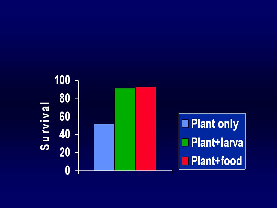
83. Cushman et al. (1994) Ecology 75:1031 -1042 Effect of different diets on survival of ants: –plant only, plant+butterfly larvae, plant+artificial ant food –three groups (treatments), 10 replicate vials of ants per treatment. Null hypothesis: –no difference in survival between groups.

85. SourcedfMSFP Diet25594.927.130.001 Residual27206.2 Reject H O

86. Independence of comparisons All pairwise comparisons not independent of each other: –e.g. pairwise comparisons of 3 means –Test 1: mean 1 significantly less than mean 2 –Test 2: mean 2 significantly less than mean 3 –Test 3: compare mean 1 to mean 3 Ho much less likely to be true given tests 1 and 2 P-value difficult to interpret