1. Hidden Variables, the EM Algorithm, and Mixtures of Gaussians Computer Vision CS 143, Brown James Hays 02/22/11 Many slides from Derek Hoiem

2. Today’s Class Examples of Missing Data Problems – Detecting outliers Background – Maximum Likelihood Estimation – Probabilistic Inference Dealing with “Hidden” Variables – EM algorithm, Mixture of Gaussians – Hard EM Slide: Derek Hoiem

3. Missing Data Problems: Outliers You want to train an algorithm to predict whether a photograph is attractive. You collect annotations from Mechanical Turk. Some annotators try to give accurate ratings, but others answer randomly. Challenge: Determine which people to trust and the average rating by accurate annotators. Photo: Jam343 (Flickr) Annotator Ratings 10 8 9 2 8

4. Missing Data Problems: Object Discovery You have a collection of images and have extracted regions from them. Each is represented by a histogram of “visual words”. Challenge: Discover frequently occurring object categories, without pre-trained appearance models. http://www.robots.ox.ac.uk/~vgg/publications/papers/russell06.pdf

5. Missing Data Problems: Segmentation You are given an image and want to assign foreground/background pixels. Challenge: Segment the image into figure and ground without knowing what the foreground looks like in advance. Foreground Background Slide: Derek Hoiem

6. Missing Data Problems: Segmentation Challenge: Segment the image into figure and ground without knowing what the foreground looks like in advance. Three steps: 1.If we had labels, how could we model the appearance of foreground and background? 2.Once we have modeled the fg/bg appearance, how do we compute the likelihood that a pixel is foreground? 3.How can we get both labels and appearance models at once? Foreground Background Slide: Derek Hoiem

7. Maximum Likelihood Estimation 1.If we had labels, how could we model the appearance of foreground and background? Foreground Background Slide: Derek Hoiem

8. Maximum Likelihood Estimation data parameters Slide: Derek Hoiem

9. Maximum Likelihood Estimation Gaussian Distribution Slide: Derek Hoiem

10. Maximum Likelihood Estimation Gaussian Distribution Slide: Derek Hoiem

11. Example: MLE >> mu_fg = mean(im(labels)) mu_fg = 0.6012 >> sigma_fg = sqrt(mean((im(labels)-mu_fg).^2)) sigma_fg = 0.1007 >> mu_bg = mean(im(~labels)) mu_bg = 0.4007 >> sigma_bg = sqrt(mean((im(~labels)-mu_bg).^2)) sigma_bg = 0.1007 >> pfg = mean(labels(:)); labelsim fg: mu=0.6, sigma=0.1 bg: mu=0.4, sigma=0.1 Parameters used to Generate Slide: Derek Hoiem

12. Probabilistic Inference 2.Once we have modeled the fg/bg appearance, how do we compute the likelihood that a pixel is foreground? Foreground Background Slide: Derek Hoiem

13. Probabilistic Inference Compute the likelihood that a particular model generated a sample component or label Slide: Derek Hoiem

14. Probabilistic Inference Compute the likelihood that a particular model generated a sample component or label Slide: Derek Hoiem

15. Probabilistic Inference Compute the likelihood that a particular model generated a sample component or label Slide: Derek Hoiem

16. Probabilistic Inference Compute the likelihood that a particular model generated a sample component or label Slide: Derek Hoiem

17. Example: Inference >> pfg = 0.5; >> px_fg = normpdf(im, mu_fg, sigma_fg); >> px_bg = normpdf(im, mu_bg, sigma_bg); >> pfg_x = px_fg*pfg./ (px_fg*pfg + px_bg*(1-pfg)); im fg: mu=0.6, sigma=0.1 bg: mu=0.4, sigma=0.1 Learned Parameters p(fg | im) Slide: Derek Hoiem

18. Figure from “Bayesian Matting”, Chuang et al. 2001 Mixture of Gaussian* Example: Matting

19. Result from “Bayesian Matting”, Chuang et al. 2001

20. Dealing with Hidden Variables 3.How can we get both labels and appearance models at once? Foreground Background Slide: Derek Hoiem

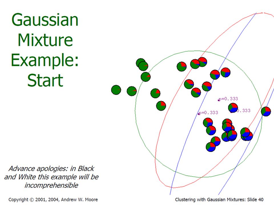
21. Mixture of Gaussians mixture component component prior component model parameters Slide: Derek Hoiem

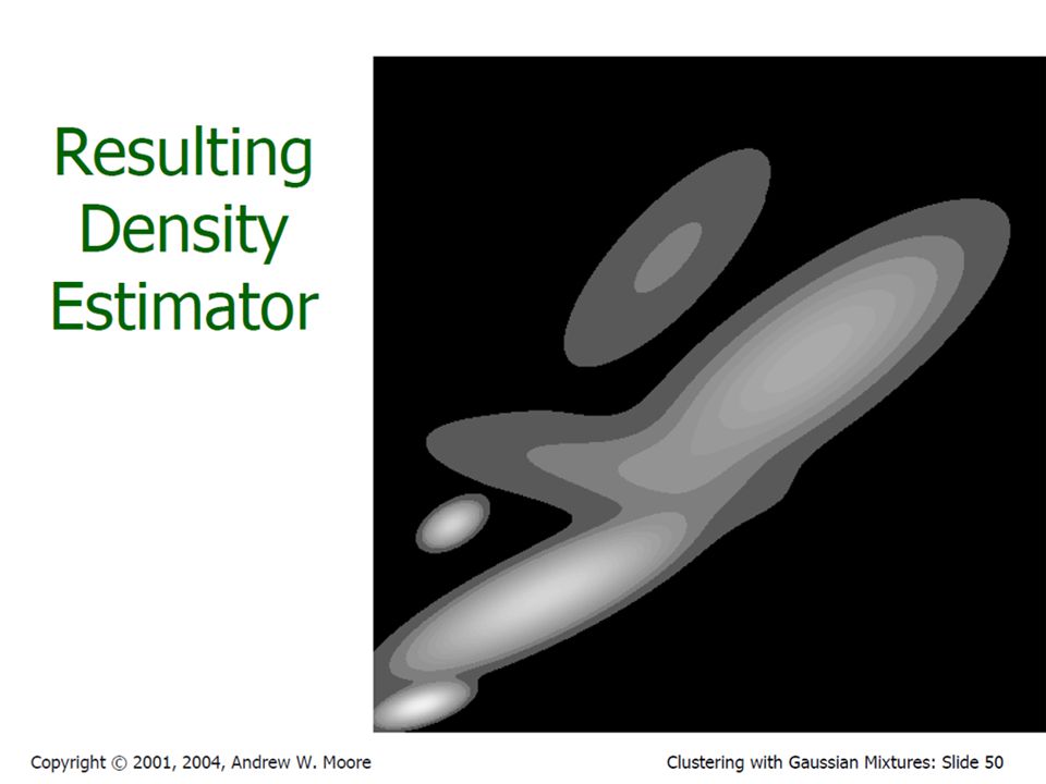
22. Mixture of Gaussians With enough components, can represent any probability density function – Widely used as general purpose pdf estimator Slide: Derek Hoiem

23. Segmentation with Mixture of Gaussians Pixels come from one of several Gaussian components – We don’t know which pixels come from which components – We don’t know the parameters for the components Slide: Derek Hoiem

24. Simple solution 1.Initialize parameters 2.Compute the probability of each hidden variable given the current parameters 3.Compute new parameters for each model, weighted by likelihood of hidden variables 4.Repeat 2-3 until convergence Slide: Derek Hoiem

25. Mixture of Gaussians: Simple Solution 1.Initialize parameters 2.Compute likelihood of hidden variables for current parameters 3.Estimate new parameters for each model, weighted by likelihood Slide: Derek Hoiem

26. Expectation Maximization (EM) Algorithm Goal: Jensen’s Inequality Log of sums is intractable See here for proof: www.stanford.edu/class/cs229/notes/cs229-notes8.pswww.stanford.edu/class/cs229/notes/cs229-notes8.ps for concave funcions, such as f(x)=log(x) Slide: Derek Hoiem

27. Expectation Maximization (EM) Algorithm 1.E-step: compute 2.M-step: solve Goal: Slide: Derek Hoiem

39. EM for Mixture of Gaussians (on board) 1.E-step: 2.M-step:

40. EM for Mixture of Gaussians (on board) 1.E-step: 2.M-step: Slide: Derek Hoiem

41. EM Algorithm Maximizes a lower bound on the data likelihood at each iteration Each step increases the data likelihood – Converges to local maximum Common tricks to derivation – Find terms that sum or integrate to 1 – Lagrange multiplier to deal with constraints Slide: Derek Hoiem

42. Mixture of Gaussian demos http://www.cs.cmu.edu/~alad/em/ http://lcn.epfl.ch/tutorial/english/gaussian/html/ Slide: Derek Hoiem

43. “Hard EM” Same as EM except compute z* as most likely values for hidden variables K-means is an example Advantages – Simpler: can be applied when cannot derive EM – Sometimes works better if you want to make hard predictions at the end But – Generally, pdf parameters are not as accurate as EM Slide: Derek Hoiem

44. Missing Data Problems: Outliers You want to train an algorithm to predict whether a photograph is attractive. You collect annotations from Mechanical Turk. Some annotators try to give accurate ratings, but others answer randomly. Challenge: Determine which people to trust and the average rating by accurate annotators. Photo: Jam343 (Flickr) Annotator Ratings 10 8 9 2 8

45. Missing Data Problems: Object Discovery You have a collection of images and have extracted regions from them. Each is represented by a histogram of “visual words”. Challenge: Discover frequently occurring object categories, without pre-trained appearance models. http://www.robots.ox.ac.uk/~vgg/publications/papers/russell06.pdf

46. What’s wrong with this prediction? P(foreground | image) Slide: Derek Hoiem

47. Next class MRFs and Graph-cut Segmentation Slide: Derek Hoiem

48. Missing data problems Outlier Detection – You expect that some of the data are valid points and some are outliers but… – You don’t know which are inliers – You don’t know the parameters of the distribution of inliers Modeling probability densities – You expect that most of the colors within a region come from one of a few normally distributed sources but… – You don’t know which source each pixel comes from – You don’t know the Gaussian means or covariances Discovering patterns or “topics” – You expect that there are some re-occuring “topics” of codewords within an image collection. You want to… – Figure out the frequency of each codeword within each topic – Figure out which topic each image belongs to Slide: Derek Hoiem

49. Running Example: Segmentation 1.Given examples of foreground and background – Estimate distribution parameters – Perform inference 2.Knowing that foreground and background are “normally distributed” 3.Some initial estimate, but no good knowledge of foreground and background