1. Shape From Light Field meets Robust PCA
Heber, Stefan, and Thomas Pock. "Shape from Light Field Meets Robust PCA." Computer Vision–ECCV Springer International Publishing,
Shape From Light Field meets Robust PCA
Jinsun Park
Good afternoon. I am Jinsun Park, in the second semester of M.S course.
The paper I am going to explain from now on is the ECCV 2014 paper, ‘Shape from light field meets robust PCA’.

2. Contents Light Field Robust PCA Ideas Algorithm Results Discussion
These are contents.

3. 1. Light Field
The light field is a function that describes the amount of light traveling in every direction, through every point in space.
𝐿 1 = 𝐿( 𝑥 1 , 𝑦 1 , 𝑧 1 , 𝜃 1 , 𝜙 1 )
𝐿 2 = 𝐿( 𝑥 2 , 𝑦 2 , 𝑧 2 , 𝜃 2 , 𝜙 2 )
( 𝑥 1 , 𝑦 1 , 𝑧 1 )
( 𝑥 2 , 𝑦 2 , 𝑧 2 ) 𝑥 𝑦 𝑧
𝜃 :𝑎𝑧𝑖𝑚𝑢𝑡ℎ 𝑎𝑛𝑔𝑙𝑒
𝜙 :𝑝𝑜𝑙𝑎𝑟 𝑎𝑛𝑔𝑙𝑒
I think I should explain first what the light field is. The light field is a function that describes position and direction of all the rays in the space.
Let’s see that smile object. It lies on Cartesian coordinate system. We can see that object because lights are reflected or emitted from its surface.
For example, there are two points on the surface of that object and two rays, let’s say, reflected from that points.
We can describe those rays by using x, y, z, azimuth and polar angle. L1 is reflected from x1, y1, z1, and its azimuth and polar angle is theta1 and phi1 respectively.
L2 can be described in same way.

4. 1. Light Field
This function can be parameterized by two parallel planes.
(Two-plane parameterization)
𝐿 1 = 𝐿( 𝑢 1 , 𝑣 1 , 𝑠 1 , 𝑡 1 )
𝐿 2 = 𝐿( 𝑢 2 , 𝑣 2 , 𝑠 2 , 𝑡 2 )
( 𝑢 1 , 𝑣 1 )
( 𝑢 2 , 𝑣 2 )
( 𝑠 1 , 𝑡 1 )
( 𝑠 2 , 𝑡 2 )
Lens Plane
(View Point)
Image Plane
(Sensor Plane)
Of course, those lights can be represented using different parameters. For example, we can assume that there exist two parallel planes between an observer and an object.
Then a ray can be described with those crossing points on two planes.
If we think about camera system, we can regard s-t plane(image plane) as sensor plane and u-v plane as lens plane.
We will use this two-plane parameterization because it’s intuitive to understand light field imaging system.

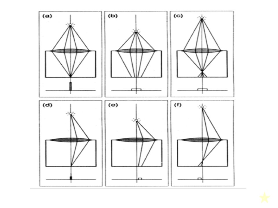
5. 1. Light Field Shifting in lens plane results in view point change.𝑢 𝑣
In camera system, we cannot move sensor plane commonly. Therefore, we can think about shifting in lens plane.
(Drawing Adelson and wang’s picture or use hidden slide) If we make a picture only using the rays from specific lens plane points, that image is equal to the image shown in front of that point. Therefore, as long as we can record those rays from each view point separately, we can get light field in a single snapshot.
This process is possible in commercial light field cameras like Lytro or Raytrix. However, the structure of those camera is not our interest. So I will skip details about structures.
The disparity of each pixel is dependent on its distance from viewpoint. (i.e. depth)
We call these images sub-aperture images.

6. 1. Light Field Shifting in lens plane results in view point change. 𝑢𝑣
Shifting in lens plane results in view point change.
Let me show you some example. These are synthetic light field images. Can you recognize changing of view point?
As you can see, disparity of each pixel depends on its distance from focal point.
For example, Mona Lisa moves a lot because it is far away from focal point. But ‘T’ moves little because it is near the focal point.
In addition, moving directions are determined by whether it is inside or outside of focal point. Their moving direction is opposite.

7. 1. Light Field Shifting in lens plane results in view point change. 𝑢𝑣
Shifting in lens plane results in view point change.

8. 1. Light Field Shifting in lens plane results in view point change. 𝑢𝑣
Shifting in lens plane results in view point change.

9. 1. Light Field Shifting in lens plane results in view point change. 𝑢𝑣
Shifting in lens plane results in view point change.

10. 1. Light Field Shifting in lens plane results in view point change. 𝑢𝑣
Shifting in lens plane results in view point change.

11. 1. Light Field Shifting in lens plane results in view point change. 𝑢𝑣
Shifting in lens plane results in view point change.

12. 1. Light Field Shifting in lens plane results in view point change. 𝑢𝑣
Shifting in lens plane results in view point change.

13. 1. Light Field Shifting in lens plane results in view point change. 𝑢𝑣
Shifting in lens plane results in view point change.

14. 1. Light Field Shifting in lens plane results in view point change. 𝑢𝑣
Shifting in lens plane results in view point change.

15. 2. Robust PCA
Let us assume that the given data lies approximately on a low dimensional subspace.
What would happen if we stack data as a row vector of a matrix M?
→ M should have low rank.
𝐿 0 :𝑙𝑜𝑤 𝑟𝑎𝑛𝑘 𝑐𝑜𝑚𝑝𝑜𝑛𝑒𝑛𝑡
𝐸 0 :𝑛𝑜𝑖𝑠𝑒
𝑀= 𝐿 0 + 𝐸 0
If we know rank 𝑟 of M, PCA provides an optimal estimate to 𝐿 0 because PCA tries to minimizes noise component 𝐸 0 .
But we don’t know 𝑟…
Next, Let’s talk about Robust PCA.
Assume that the given data is approximately on a low dimensional subspace. It means that there exist redundant dimension in data.
What would happen if we make a matrix by stacking these data row or column wise?
M should have low rank.
So we can decompose M into low rank component and noise component.
If we know rank r ahead, this decomposition can be done by means of PCA.
But we don’t know r…

16. min 𝐿, 𝐸 𝑟𝑎𝑛𝑘 𝐿 + 𝜇 𝐸 0 subject to 𝑀=𝐿+𝐸
2. Robust PCA
𝐿 0 :𝑙𝑜𝑤 𝑟𝑎𝑛𝑘 𝑐𝑜𝑚𝑝𝑜𝑛𝑒𝑛𝑡
𝐸 0 :𝑛𝑜𝑖𝑠𝑒
𝑀= 𝐿 0 + 𝐸 0
Candès et al.1) suggested an efficient algorithm which extracts principal components in the presence of sparse errors with unknown matrix rank.
min 𝐿, 𝐸 𝑟𝑎𝑛𝑘 𝐿 + 𝜇 𝐸 subject to 𝑀=𝐿+𝐸
where ∙ 0 denotes 𝐿 0 norm. (the number of non zero entries)
→ Unfortunately, this combinatorial problem is NP-hard.
→ We need convex relaxation.
Candes et al. suggested an efficient algorithm to decompose those components with unknown rank r.
The objective function of this algorithm is like this.
L0 norm is nothing but the number of non zero entries.
Unfortunately, this problem is NP-hard. Briefly speaking, NP-hard problems cannot be solved in polynomial time and require exponential time.
So it’s almost infeasible to solve this problem as it is.
Therefore, we need convex relaxation to solve this problem.
1) Candès, Emmanuel J., et al. "Robust principal component analysis?." Journal of the ACM (JACM) 58.3 (2011): 11.

17. 𝜎 𝑖 𝑋 : i-th singular value ( 𝜎 1 𝑋 ≥ 𝜎 2 𝑋 ≥⋯≥ 𝜎 𝑛 𝑋 ≥0)
2. Robust PCA
In energy minimization problem, almost all functionals are non-convex and NP-hard.
Convex relaxation methods aim to solve these problems by approximating the given functionals by convex ones.
𝑟𝑎𝑛𝑘 ∙ → ∙ ∗
∙ 0 → ∙ 1
where ∙ ∗ denotes Nuclear norm and ∙ 1 denotes 𝐿 1 norm.
※ Nuclear Norm1)
𝑋 ∗ = 𝑖=1 𝑛 𝜎 𝑖 (𝑋)
where
𝑋∈ 𝑅 𝑛 1 × 𝑛 2
𝑛 ≔min⁡{ 𝑛 1 , 𝑛 2 }
𝜎 𝑖 𝑋 : i-th singular value ( 𝜎 1 𝑋 ≥ 𝜎 2 𝑋 ≥⋯≥ 𝜎 𝑛 𝑋 ≥0)
1) Nuclear norm can be interpreted as the 𝐿 1 norm of the vector of singular values of X.
Convex relaxation is approximation of non-convex and NP-hard problems using convex functions.
In previous objective function, there were rank function and L0 norm.
We take nuclear norm as an alternative to rank function and L1 norm to approximate L0 norm because they are convex and known as reasonable approximations of those functions.
I think you know L1 norm. So I will not talk about L1 norm.
The Nuclear norm is defined by this equation. It is easier to regard this one as the L1 norm of the singular values of matrix X.

18. 2. Robust PCA min 𝐿, 𝐸 𝑟𝑎𝑛𝑘 𝐿 + 𝜇 𝐸 0 subject to 𝑀=𝐿+𝐸
We will use this energy functional for our data term of objective function.
With those convex functions, we can obtain convex relaxation of objective function. This term will be used as a data term in our final objective function.

19. Matrix M with those images
3. Ideas
The point correspondences between an image and a reference image (e.g. center view) is closely related to the depth information. So we will try to find best warping to determine depth information.
Furthermore, if we warp an image exactly to a reference image, two image will be identical.
Matrix M with those images
I am going to talk about the authors’ idea from now on.
The key idea of this paper is that if we know exact point correspondences of two images, we can warp one image to the other image perfectly. This process will result in two identical images.
In general, if we have some images we can warp those images to the common warping center(e.g. center view) and a matrix constructed from stacking of those image will have row rank.
→ M will have low rank.

20. 3. Ideas
We can construct objective function by combining those ideas previously explained.
min 𝑢,𝐿 𝜇 𝐿 ∗ + 𝜆 𝐿 −𝐼 𝑢 𝑅 𝑢 subject to 𝐼 𝑢 =𝐿+𝑆
𝑢 : disparity
𝐼 𝑢 : matrix whose i-th row is vectorized i-th sub-aperture image
𝜇, 𝜆 : modeling parameters (> 0)
𝑅 𝑢 : regularization term
From this idea, we can construct objective function like this. U is disparity, I is constructed matrix, mu and lambda are parameters and R is regularization term.
The term (L-I) in L1 norm came from constraint. (I = L+S)

21. 3. Ideas
A reliable solution of disparity is piecewise smooth one. We model this assumption by defining 𝑅 𝑢 to be the 2nd order Total Generalized Variation(TGV).
𝑅 𝑢 ≔ min 𝑤 𝛼 1 𝛻𝑢 −𝑤 𝑀 + 𝛼 0 𝜵𝑤 𝑀
∙ 𝑀 : Radon norm1)
𝛼 0 , 𝛼 1 : parameters
𝛻, 𝜵 : first and second order gradient operator
For the regularization term, the authors adopted total generalized variation. It is a generalized version of total variation.
N-th order TGV favors (n-1)-th continuous solutions. Because we want piecewise smooth solutions, 2nd order TGV will be our choice.
TGV2 can be defined by this equation. This norm means radon norm. Honestly, I don’t fully understand what the radon norm is although I tried hard to understand it. With a help of Wikipedia, I found out that it comes from measure theory.
I searched a lot of papers to figure out how to deal with it. Fortunately, the result was simple. In many papers, it is just calculated by summation of gradients.
This objective function can be interpreted like this way. W is related to the gradient of u. So we can regard w as the 1st derivatives and del(w) as the 2nd derivatives. The first term serves as a data term and the second term does as a regularization term. In this sense, because the 2nd derivative is regularized, the 1st derivative will be piecewise constant which means solution is piecewise linear.
(If needed, draw picture)
1) In many reference papers, radon norm is simply calculated by summation of gradients.

22. 3. Ideas
Each sub-aperture images can be approximated by first order Taylor expansion.
𝐼 𝑖 𝑢 ≔ 𝐿 𝒑 − 𝑢 𝒑 𝜑 𝑖 𝑅 , 𝜑 𝑖
𝐿 : Light field
𝑝 : Image plane coordinates
𝜑 𝑖 : directional offset
𝑅 : maximum offset distance
𝐿 𝒑 − 𝑢 𝒑 𝜑 𝑖 𝑅 , 𝜑 𝑖
≈ 𝐿 𝒑 − 𝑢 0 𝒑 𝜑 𝑖 𝑅 , 𝜑 𝑖 + 𝑢 𝒑 − 𝑢 0 𝒑 𝜑 𝑖 𝑅 𝛻 − 𝜑 𝑖 𝜑 𝑖 𝐿 𝒑 − 𝑢 0 𝒑 𝜑 𝑖 𝑅 , 𝜑 𝑖
= 𝐵 𝑖 + 𝐴 𝑖 𝑢 𝒑 − 𝑢 0 𝒑
𝛻 𝑣 : directional derivative
Warping sub-aperture image can be approximated by the 1st order Taylor expansion because the first order approximation is enough in this case.
(Use blackboard to explain first order Taylor expansion)
Del sub v(del_v) denotes a directional derivative.
(Draw directional derivative on blackboard)

23. 4. Algorithm Objective function is as follows:
min 𝑢,𝐿 𝜇 𝐿 ∗ + 𝜆 𝑖=1 𝑀 𝑙 𝑖 𝑇 − 𝑏 𝑖 − 𝐴 𝑖 𝑢 − 𝑢 𝑅 𝑢
𝑙 𝑖 : i-th row of L
𝑏 𝑖 : vectorized 𝐵 𝑖
𝐴 𝑖 : diagonalized matrix of vectorized 𝐴 𝑖
To reformulate the problem into a saddle-point problem, we introduce the dual variables and obtain the following formulation.
min 𝑢,𝑤,𝐿 max 𝑝 𝑢 ∞ ≤1 𝑝 𝑤 ∞ ≤1 𝑝 𝑖 ∞ ≤1 𝜇 𝐿 ∗ + 𝜆 𝑖=1 𝑀 𝑙 𝑖 𝑇 − 𝑏 𝑖 − 𝐴 𝑖 𝑢− 𝑢 0 , 𝑝 𝑖 + 𝛼 1 𝛻𝑢 −𝑤, 𝑝 𝑢 + 𝛼 0 𝜵𝑤, 𝑝 𝑤
Final objective function is like this. The difference between L and sub-aperture images are expressed by summation operator.
In order to make the problem saddle point problem, we introduce dual variables P_u, P_i, and P_w.
Angle brackets denotes standard inner product.

24. 4. Algorithm
The saddle point problem can be solved by using Primal-Dual algorithm. In Primal-Dual algorithm, we solve primal and dual problems alternately.
By alternately solving those problems, we are able to get the optimal solution.
(id + tau*mu/lambda) is proximal operator. It gives us a proximal point.
Simply speaking, a proximal point is a point which compromises between minimizing objective function and being near to the given value. (Use blackboard or hidden slide)
In the paper, authors took iterative and coarse-to-fine approach. This means that we start from down sampled image and increase image size gradually during iteration.

25. 5. Results
Here are some results in this paper. According to authors’ comments, they outperformed state-of-the-art algorithms.

26. 5. Results
Here are comparisons to the other methods. This values represents ratio of pixels have errors more than 0.2%.

27. 5. Results Synthetic Light field center view 4 2 Ground truth
This is result from my implementation using synthetic light field image. Actually, this algorithm does not work well in plain regions.
To make this algorithm work properly, there should be textures. So I generated textured synthetic light field images.
Lower left image shows ground truth depth where true disparity values are shown. Lower right one shows result from implemented algorithm. Although there exist some errors, it works well with textured image.
It took 106 sec to calculate 25 scale level with 15 iteration for each scale level. Image size is 200 by 200. 2
Ground truth
Optimization result
Process time : 106 sec, Iteration : 15, Scale Level : 25

28. 5. Results Ground truth Optimization result
Result shown as 3d plot. Shows reasonable results.

29. 5. Results Error larger than 0.3 pixel : 3411/40000 = 0.0853
Because of the effect of TGV2 regularization, solution tends to have smoother boundaries. This cause errors on boundary area.
The ratio of pixels which have error larger than 0.3 pixel is about 8.53%. 0.3 pixel error is about 10% of average disparity.
Honestly, this result is inferior to the authors’ results.
Error larger than 0.3 pixel : 3411/40000 =

30. 5. Results Image from light field dataset Ground truth
This is failure case. Because most parts of image are plain region, proposed algorithm failed to obtain reasonable solution.
Ground truth
Optimization result

31. 6. Discussion Pros - Can perform all vs. all matching.
- Optimization can be easily conducted.
- Coarse-to-fine approach
Cons
- Can be applied only small disparities.
- It does not work well on small gradients.
- Because of TGV, edge disparities are smoothed.
Future Works
- Extension to large disparities.
- Edge-aware regularization
- Guided filtering / Edge-preserving filtering
Summary.
The first advantage of this algorithm is that all vs. all matching is implicitly performed.
Second, objective function is not difficult to compute. Although I didn’t mention details in algorithm part, nuclear norm minimization can be calculated by soft spectral thresholding. The other terms also can be easily computed.
Furthermore, coarse-to-fine approach enables us to be able to find wide range of disparity values.
On the contrary, It doesn’t work well with large disparities. It has some limitations because this algorithm aims to solve problems in light field case where disparities are relatively small.
The major limitation of this problem is that it easily fails to find solution on plain regions because it cannot find its exact correspondence in plane region of the other image.
In addition, because TGV favors piecewise linear solutions, sharp edges are smoothed. This also make large errors in edge region.
In order to avoid those problems, we have to change regularization terms which can deal with sharp edges. For example, total variation.
Guided filtering or edge-preserving filtering can be post-processing for this problem. For example, bilateral filtering.

32. Reference
Heber, Stefan, and Thomas Pock. "Shape from Light Field Meets Robust PCA." Computer Vision–ECCV Springer International Publishing,
Heber, Stefan, Rene Ranftl, and Thomas Pock. "Variational Shape from Light Field." Energy Minimization Methods in Computer Vision and Pattern Recognition. Springer Berlin Heidelberg, 2013.
Brox, Thomas, et al. "High accuracy optical flow estimation based on a theory for warping." Computer Vision-ECCV Springer Berlin Heidelberg,
Knoll, Florian, et al. "Second order total generalized variation (TGV) for MRI."Magnetic resonance in medicine 65.2 (2011):
Bredies, Kristian, Karl Kunisch, and Thomas Pock. "Total generalized variation." SIAM Journal on Imaging Sciences 3.3 (2010):
Candès, Emmanuel J., et al. "Robust principal component analysis?." Journal of the ACM (JACM) 58.3 (2011): 11.

33. Q & A
Thank you!
Thank you for listening. Please feel free to ask questions.