1. 9.2 The Traveling Salesman Problem

2. Let us return to the question of finding a cheapest possible cycle through all the given towns: We have n towns (points) in the plane, and for any two of them we are given the “cost” of connecting them directly. We have to find a cycle with these nodes such that the cost of the cycle (the sum of the costs of its edges) is as small as possible.

3. This problem is one of the most important in the area of combinatorial optimization, the field dealing with finding the best possible design in various combinatorial situations, like finding the optimal tree discussed in the previous section.

4. Traveling Salesman Problem Its name comes from the version of the problem where a traveling salesman has to visit all towns in a region and then return to his home, and of course, he wants to minimize his travel costs. It is clear that mathematically, this is the same problem. It is easy to imagine that one and the same mathematical problem appears in connection with designing optimal delivery routes for mail, optimal routes for garbage collection, etc.

5. The following important question leads to the same mathematical problem, except on an entirely different scale. A machine has to drill a number of holes in a printed circuit board (this number could be in the thousands),and then return to the starting point. In this case, the important quantity is the time it takes to move the drilling head from one hole to the next, since the total time a given board has to spend on the machine determines the number of boards that can be processed in a day. So if we take the time needed to move the head from one hole to another as the “cost” of this edge, we need to find a cycle with the holes as nodes, and with minimum cost.

6. The Traveling Salesman Problem is closely related to Hamiltonian cycles. First of all, a traveling salesman tour is just a Hamiltonian cycle in the complete graph on the given set of nodes. But there is a more interesting connection: The problem of whether a given graph has a Hamiltonian cycle can be reduced to the Traveling Salesman Problem.

7. Let G be a graph with n nodes. We define the “distance” of two nodes as follows: adjacent nodes have distance 1; nonadjacent nodes have distance 2. What do we know about the Traveling Salesman Problem on the set of nodes of G with this new distance function? If the graph contains a Hamiltonian cycle, then this is a traveling salesman tour of length n. If the graph has no Hamiltonian cycle, then the shortest traveling salesman tour has length at least n + 1.

8. This shows that any algorithm that solves the Traveling Salesman Problem can be used to decide whether or not a given graph has a Hamiltonian cycle.

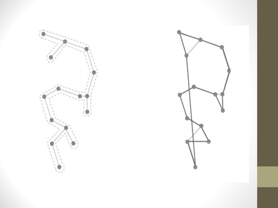
10. So we find the cheapest tree T, with total cost c. One thing we can do is to walk around the tree just as we did when constructing the “planar code” of a tree in the proof of Theorem 8.5.1 (see Figure 8.6). This certainly gives a walk that goes through each town at least once, and returns to the starting point. Of course, this walk may pass through some of the towns more than once. But this is good for us: We can make shortcuts. If the walk takes us from I to j to k, and we have seen j already, we can proceed directly from i to k. Doing such shortcuts as long as we can, we end up with a tour that goes through every town exactly once (Figure 9.3). Let us call the algorithm described above the Tree Shortcut Algorithm.

12. Theorem 9.2.1 If the costs in a Traveling Salesman Problem satisfy the triangle inequality, then the Tree Shortcut Algorithm finds a tour that costs less than twice as much as the optimum tour.

13. Proof The cost of the walk around the tree is exactly twice the cost c of T, since we used every edge twice. The triangle inequality guarantees that we have only shortened our walk by doing shortcuts, so the cost of the tour we found is not more than twice the cost of the cheapest spanning tree.

14. But we want to relate the cost of the tour we obtained to the cost of the optimum tour, not to the cost of the optimum spanning tree! Well, this is easy now: The cost of a cheapest spanning tree is always less than the cost of the cheapest tour. Why? Because we can omit any edge of the cheapest tour to get a spanning tree. This is a very special kind of tree (a path),and as a spanning tree it mayor may not be optimal. However, its cost is certainly not smaller than the cost of the cheapest tree, but smaller than the cost of the optimal tour, which proves the assertion above.

15. Since d>e>c and c’<2c So c’<2d

16. To sum up, the cost of the tour we constructed is at most twice that of the cheapest spanning tree, which in turn is less than twice the cost of a cheapest tour.