1. Statistics 101 & Exploratory Data Analysis (EDA)

2. A definition of probability
Consider a set S with subsets A, B, ...
Kolmogorov
axioms (1933)
From these axioms we can derive further properties, e.g.

3. Conditional probability, independence
Also define conditional probability of A given B (with P(B) ≠ 0):
E.g. rolling dice:
Subsets A, B independent if:
If A, B independent,
N.B. do not confuse with disjoint subsets, i.e.,

4. Interpretation of probability
I. Relative frequency
A, B, ... are outcomes of a repeatable experiment
cf. quantum mechanics, particle scattering, radioactive decay...
II. Subjective probability
A, B, ... are hypotheses (statements that are true or false)
• Both interpretations consistent with Kolmogorov axioms.
• In particle physics frequency interpretation often most useful,
but subjective probability can provide more natural treatment of
non-repeatable phenomena:
systematic uncertainties, probability that Higgs boson exists,...

5. Bayes’ theorem From the definition of conditional probability we have,
and
but
, so
Bayes’ theorem
First published (posthumously) by the
Reverend Thomas Bayes (1702−1761)
An essay towards solving a problem in the
doctrine of chances, Philos. Trans. R. Soc. 53
(1763) 370; reprinted in Biometrika, 45 (1958) 293.

6. The law of total probability
Consider a subset B of
the sample space S, S
divided into disjoint subsets Ai
such that ∪i Ai = S, Ai
B ∩ Ai → → →
law of total probability
Bayes’ theorem becomes

7. An example using Bayes’ theorem
Suppose the probability (for anyone) to have AIDS is:
← prior probabilities, i.e.,
before any test carried out
Consider an AIDS test: result is + or -
← probabilities to (in)correctly
identify an infected person
← probabilities to (in)correctly
identify an uninfected person
Suppose your result is +. How worried should you be?

8. Bayes’ theorem example (cont.)
The probability to have AIDS given a + result is
← posterior probability
i.e. you’re probably OK!
Your viewpoint: my degree of belief that I have AIDS is 3.2%
Your doctor’s viewpoint: 3.2% of people like this will have AIDS

9. Frequentist Statistics − general philosophy
In frequentist statistics, probabilities are associated only with
the data, i.e., outcomes of repeatable observations (shorthand: ).
Probability = limiting frequency
Probabilities such as
P (AIDS exists),
P (0.117 < as < 0.121),
etc. are either 0 or 1, but we don’t know which.
The tools of frequentist statistics tell us what to expect, under
the assumption of certain probabilities, about hypothetical
repeated observations.
The preferred theories (models, hypotheses, ...) are those for which our observations would be considered ‘usual’.

10. Bayesian Statistics − general philosophy
In Bayesian statistics, use subjective probability for hypotheses:
probability of the data assuming
hypothesis H (the likelihood)
prior probability, i.e.,
before seeing the data
posterior probability, i.e.,
after seeing the data
normalization involves sum
over all possible hypotheses
Bayes’ theorem has an “if-then” character: If your prior
probabilities were p (H), then it says how these probabilities
should change in the light of the data.
No general prescription for priors (subjective!)

11. Random variables and probability density functions
A random variable is a numerical characteristic assigned to an element of the sample space; can be discrete or continuous.
Suppose outcome of experiment is continuous value x
→ f(x) = probability density function (pdf)
x must be somewhere
Or for discrete outcome xi with e.g. i = 1, 2, ... we have
probability mass function
x must take on one of its possible values

12. Cumulative distribution function
Probability to have outcome less than or equal to x is
cumulative distribution function
Alternatively define pdf with

13. Histograms pdf = histogram with infinite data sample, zero bin width,
normalized to unit area.

14. Multivariate distributions
Outcome of experiment charac-
terized by several values, e.g. an
n-component vector, (x1, ... xn)
joint pdf
Normalization:

15. Marginal pdf Sometimes we want only pdf of
some (or one) of the components: i
→ marginal pdf
x1, x2 independent if

16. Marginal pdf (2)
Marginal pdf ~ projection of joint pdf onto individual axes.

17. Conditional pdf
Sometimes we want to consider some components of joint pdf as constant. Recall conditional probability:
→ conditional pdfs:
Bayes’ theorem becomes:
Recall A, B independent if
→ x, y independent if

18. Conditional pdfs (2)
E.g. joint pdf f(x,y) used to find conditional pdfs h(y|x1), h(y|x2):
Basically treat some of the r.v.s as constant, then divide the joint
pdf by the marginal pdf of those variables being held constant so
that what is left has correct normalization, e.g.,

19. Expectation values Consider continuous r.v. x with pdf f (x).
Define expectation (mean) value as
Notation (often): ~ “centre of gravity” of pdf.
For a function y(x) with pdf g(y),
(equivalent)
Variance:
Notation:
Standard deviation:
s ~ width of pdf, same units as x.

20. Covariance and correlation
Define covariance cov[x,y] (also use matrix notation Vxy) as
Correlation coefficient (dimensionless) defined as
If x, y, independent, i.e.,
, then →
x and y, ‘uncorrelated’
N.B. converse not always true.

21. Correlation (cont.)

22. Some distributions Distribution/pdf Binomial Multinomial Uniform
Gaussian

23. Binomial distribution
Consider N independent experiments (Bernoulli trials):
outcome of each is ‘success’ or ‘failure’,
probability of success on any given trial is p.
Define discrete r.v. n = number of successes (0 ≤ n ≤ N).
Probability of a specific outcome (in order), e.g. ‘ssfsf’ is
But order not important; there are
ways (permutations) to get n successes in N trials, total
probability for n is sum of probabilities for each permutation.

24. Binomial distribution (2)
The binomial distribution is therefore
random
variable
parameters
For the expectation value and variance we find:

25. Binomial distribution (3)
Binomial distribution for several values of the parameters:
Example: observe N decays of W±, the number n of which are
W→mn is a binomial r.v., p = branching ratio.

26. Multinomial distribution
Like binomial but now m outcomes instead of two, probabilities are
For N trials we want the probability to obtain:
n1 of outcome 1,
n2 of outcome 2, 
nm of outcome m.
This is the multinomial distribution for

27. Multinomial distribution (2)
Now consider outcome i as ‘success’, all others as ‘failure’.
→ all ni individually binomial with parameters N, pi
for all i
One can also find the covariance to be
Example:
represents a histogram
with m bins, N total entries, all entries independent.

28. Uniform distribution
Consider a continuous r.v. x with -∞ < x < ∞ . Uniform pdf is:
N.B. For any r.v. x with cumulative distribution F(x),
y = F(x) is uniform in [0,1].
Example: for p0 → gg, Eg is uniform in [Emin, Emax], with

29. Gaussian distribution
The Gaussian (normal) pdf for a continuous r.v. x is defined by:
(N.B. often m, s2 denote
mean, variance of any
r.v., not only Gaussian.)
Special case: m = 0, s2 = 1 (‘standard Gaussian’):
If y ~ Gaussian with m, s2, then x = (y - m) /s follows  (x).

30. Gaussian pdf and the Central Limit Theorem
The Gaussian pdf is so useful because almost any random
variable that is a sum of a large number of small contributions
follows it. This follows from the Central Limit Theorem:
For n independent r.v.s xi with finite variances si2, otherwise
arbitrary pdfs, consider the sum
In the limit n → ∞, y is a Gaussian r.v. with
Measurement errors are often the sum of many contributions, so frequently measured values can be treated as Gaussian r.v.s.

31. Multivariate Gaussian distribution
Multivariate Gaussian pdf for the vector
are column vectors,
are transpose (row) vectors,
For n = 2 this is
where r = cov[x1, x2]/(s1s2) is the correlation coefficient.

32. Univariate Normal Distribution

33. Multivariate Normal Distribution

34. Random Sample and Statistics
Population: is used to refer to the set or universe of all entities under study.
However, looking at the entire population may not be feasible, or may be too expensive.
Instead, we draw a random sample from the population, and compute appropriate statistics from the sample, that give estimates of the corresponding population parameters of interest.

35. Statistic
Let Si denote the random variable corresponding to data point xi , then a statistic ˆθ is a function ˆθ : (S1, S2, · · · , Sn) → R.
If we use the value of a statistic to estimate a population parameter, this value is called a point estimate of the parameter, and the statistic is called as an estimator of the parameter.

36. Empirical Cumulative Distribution Function
Where
Inverse Cumulative Distribution Function

37. Example

38. Measures of Central Tendency (Mean)
Population Mean:
Sample Mean (Unbiased, not robust):

39. Measures of Central Tendency (Median)
Population Median: or
Sample Median:

40. Example

41. Measures of Dispersion (Range)
Sample Range:
Not robust, sensitive to extreme values

42. Measures of Dispersion (Inter-Quartile Range)
Inter-Quartile Range (IQR):
Sample IQR:
More robust

43. Measures of Dispersion (Variance and Standard Deviation)

44. Measures of Dispersion (Variance and Standard Deviation)
Sample Variance & Standard Deviation:

45. EDA and Visualization
Exploratory Data Analysis (EDA) and Visualization are important (necessary?) steps in any analysis task.
get to know your data!
distributions (symmetric, normal, skewed)
data quality problems
outliers
correlations and inter-relationships
subsets of interest
suggest functional relationships
Sometimes EDA or viz might be the goal!

46. flowingdata.com 9/9/11

47. NYTimes 7/26/11

48. Exploratory Data Analysis (EDA)
Goal: get a general sense of the data
means, medians, quantiles, histograms, boxplots
You should always look at every variable - you will learn something!
data-driven (model-free)
Think interactive and visual
Humans are the best pattern recognizers
You can use more than 2 dimensions!
x,y,z, space, color, time….
especially useful in early stages of data mining
detect outliers (e.g. assess data quality)
test assumptions (e.g. normal distributions or skewed?)
identify useful raw data & transforms (e.g. log(x))
Bottom line: it is always well worth looking at your data!

49. Summary Statistics not visual sample statistics of data X
mean:  = i Xi / n
mode: most common value in X
median: X=sort(X), median = Xn/2 (half below, half above)
quartiles of sorted X: Q1 value = X0.25n , Q3 value = X0.75 n
interquartile range: value(Q3) - value(Q1)
range: max(X) - min(X) = Xn - X1
variance: 2 = i (Xi - )2 / n
skewness: i (Xi - )3 / [ (i (Xi - )2)3/2 ]
zero if symmetric; right-skewed more common (what kind of data is right skewed?)
number of distinct values for a variable (see unique() in R)
Don’t need to report all of thses: Bottom line…do these numbers make sense???

50. Single Variable Visualization
Histogram:
Shows center, variability, skewness, modality,
outliers, or strange patterns.
Bins matter
Beware of real zeros

51. Issues with Histograms
For small data sets, histograms can be misleading.
Small changes in the data, bins, or anchor can deceive
For large data sets, histograms can be quite effective at illustrating general properties of the distribution.
Histograms effectively only work with 1 variable at a time
But ‘small multiples’ can be effective

52. But be careful with axes and scales!

53. Smoothed Histograms - Density Estimates
Kernel estimates smooth out the contribution of each datapoint over a local neighborhood of that point.
h is the kernel width
Gaussian kernel is common:

54. Data Mining 2011 - Volinsky - Columbia University
Bandwidth choice is an art
Usually want to try several
Data Mining Volinsky - Columbia University

55. Boxplots Shows a lot of information about a variable in one plot
Median
IQR
Outliers
Range
Skewness
Negatives
Overplotting
Hard to tell distributional shape
no standard implementation in software (many options for whiskers, outliers)

56. summer bifurcations in air travel
Time Series
If your data has a temporal component, be sure to exploit it
summer bifurcations in air travel
(favor early/late)
summer
peaks
steady growth
trend
New Year bumps

57. Spatial Data
If your data has a geographic component, be sure to exploit it
Data from cities/states/zip cods – easy to get lat/long
Can plot as scatterplot

58. Spatio-temporal data spatio-temporal data
(Nathan Yau)
But, fancy tools not needed! Just do successive scatterplots to (almost) the same effect

59. Spatial data: choropleth Maps
Maps using color shadings to represent numerical values are called chloropleth maps

60. Two Continuous Variables
For two numeric variables, the scatterplot is the obvious choice
interesting?

61. 2D Scatterplots useful to answer:
x,y related?
linear
quadratic
other
variance(y) depend on x?
outliers present?
standard tool to display relation between 2 variables
e.g. y-axis = response, x-axis = suspected indicator
interesting?

62. Scatter Plot: No apparent relationship

63. Scatter Plot: Linear relationship

64. Scatter Plot: Quadratic relationship

65. Scatter plot: Homoscedastic
Why is this important in classical statistical modelling?

66. Scatter plot: Heteroscedastic
variation in Y differs depending on the value of X
e.g., Y = annual tax paid, X = income

67. Two variables - continuous
Scatterplots
But can be bad with lots of data

68. Two variables - continuous
What to do for large data sets
Contour plots

69. Two Variables - one categorical
Side by side boxplots are very effective in showing differences in a quantitative variable across factor levels
tips data
do men or women tip better
orchard sprays
measuring potency of various orchard sprays in repelling honeybees

70. Barcharts and Spineplots
stacked barcharts can be used to compare continuous values across two or more categorical ones.
spineplots show proportions well, but can be hard to interpret
orange=M blue=F

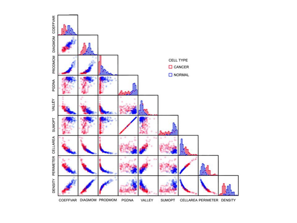
71. More than two variables
Pairwise scatterplots
Can be somewhat ineffective for categorical data
Data Mining Volinsky - Columbia University

73. Data Mining 2011 - Volinsky - Columbia University
Networks and Graphs
Visualizing networks is helpful, even if is not obvious that a network exists
Data Mining Volinsky - Columbia University

74. Network Visualization
Graphviz (open source software) is a nice layout tool for big and small graphs

75. What’s missing? pie charts 3D very popular
good for showing simple relations of proportions
Human perception not good at comparing arcs
barplots, histograms usually better (but less pretty) 3D
nice to be able to show three dimensions
hard to do well
often done poorly
3d best shown through “spinning” in 2D
uses various types of projecting into 2D

76. Dimension Reduction
One way to visualize high dimensional data is to reduce it to 2 or 3 dimensions
Variable selection
e.g. stepwise
Principle Components
find linear projection onto p-space with maximal variance
Multi-dimensional scaling
takes a matrix of (dis)similarities and embeds the points in p-dimensional space to retain those similarities

77. Fisher’s IRIS data Four features sepal length sepal width petal length
petal width
Three classes (species of iris)
setosa
versicolor
virginica
50 instances of each

78. Iris Data: http://archive.ics.uci.edu/ml/datasets/Iris
Petal, a non-reproductive part of the flower
Sepal, a non-reproductive part of the flower
The famous iris data!

80. Features 1 and 2 (sepal width/length)
Circle = setosa
Features 1 and 2 (sepal width/length)

81. Features 3 and 4 (petal width/length)

82. Homework 1 (Due Jan. 27th) Write a Java program to compute
The average, median, 25% percentile & 75% percentile and variance of each attribute of Iris data (
The histogram of each attribute (equal-interval with 10 bins)
Write a Java program to perform “permutation”: given N and k, list all the permutations
For example, N=4, k=3: 123, 124, 132, 134, 142, 143, 213, 214, … 432 (there are 24 of them)