1. Particle Flow Template Modular Particle Flow for the ILC Purity/Efficiency-based PFA PFA Module Reconstruction Jet Reconstruction Stephen Magill Argonne National Laboratory

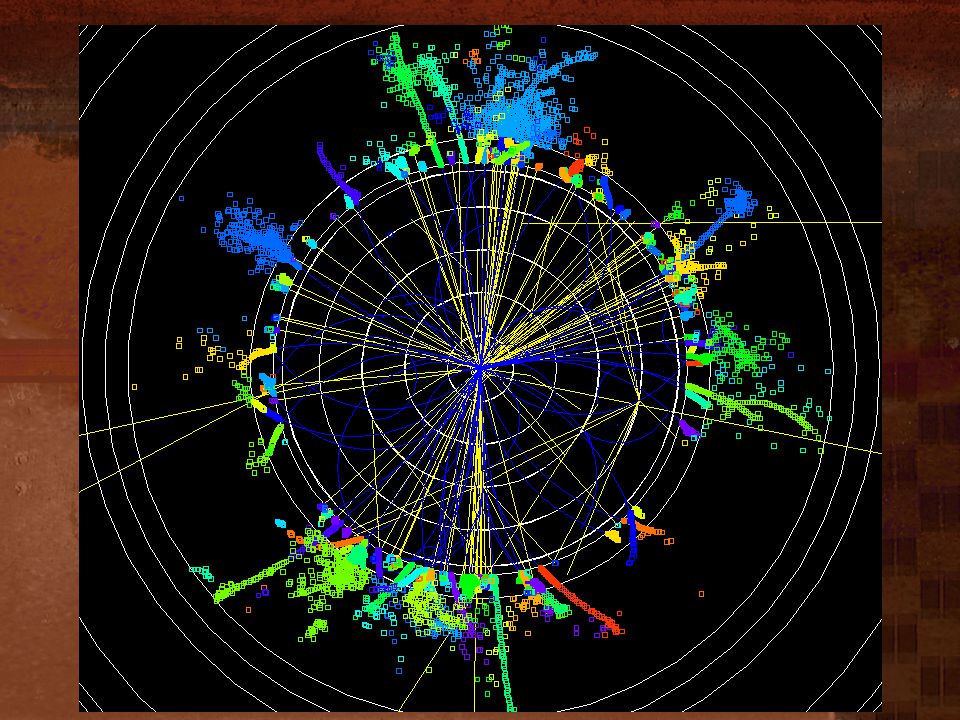
2. e + e - -> ttbar -> 6 jets @500 GeV CM

3. Parton Measurement via Jet Reconstruction From J. Kvita at CALOR06 Cal Jet -> large correction -> Particle Jet -> small correction -> Parton Jet

4. Flexible structure for PFA development based on “Hit Collections” (ANL, SLAC, Iowa) Simulated EMCAL, HCAL Hits (SLAC) DigiSim (NIU) X-talk, Noise, Thresholds, Timing, etc. EMCAL, HCAL Hit Collections Track-Mip Match Algorithm (ANL) Modified EMCAL, HCAL Hit Collections MST Cluster Algorithm (Iowa) H-Matrix algorithm (SLAC, Kansas) -> Photons Modified EMCAL, HCAL Hit Collections Nearest-Neighbor Cluster Algorithm (SLAC, NIU) Track-Shower Match Algorithm (ANL) -> Tracks Modified EMCAL, HCAL Hit Collections Nearest-Neighbor Cluster Algorithm (SLAC, NIU) Neutral ID Algorithm (SLAC, ANL) -> Neutral hadrons Modified EMCAL, HCAL Hit Collections Post Hit/Cluster ID (leftover hits?) Tracks, Photons, Neutrals to jet algorithm PFA Template – Modular Approach

5. A Systematic PFA Development Starting Point : 100% pure calorimeter cell population – 1 and only 1 particle contributes to a cell More practically, no overlap between charged particles and neutrals -> Defines cell volume – v(d IP,η,B?) -> Start of detector design optimization -> Perfect PFA is really perfect – no confusion to start 100% pure tracker hits (or obvious crossings) -> Defines Si strip size -> Start of design optimization -> Perfect Tracks are really perfect PFA is an intelligent mixture of high purity and high efficiency objects – not necessarily both together

6. Occupancy Event Display All hits from all particles Hits with >1 particle contributing

7. Standard Perfect PFA (Perfect Reconstructed Particles) Takes generated and simulated MC objects, applies rules to define what a particular detector should be able to detect, forms a list of the perfect reconstructed particles, perfect tracks, and perfect calorimeter clusters. Complicated examples : -> charged particle interactions/decays before cal -> photon conversions -> backscattered particles Critical for comparisons when perfect (cheated) tracks are used Extremely useful for debugging PFA Standard Detector Calibration Default detector calibration done with single particles Basic Clusters contain calibrated energies – analog in ECAL and digital in HCAL Standard for all SiD variants with analog ECAL, digital HCAL Checked with Perfect PFA particles

8. SiD (SS/RPC) e + e - -> Z( ) Z(qq) @ 500 GeV Perfect Tracks Perfect Neutrals (photons, neutral hadrons) Perfect Cal Clusters Perfect PFA

9. Perfect PFA – SiD01 e + e - -> qq @ 200 GeV rms90 = 3.63 GeV rms90 = 3.36 GeV 25%/  E24%/  M

10. Photons from Perfect PFA (ZPole events in ACME0605 W/Scin HCAL)  /mean ~ 18%/  E  /mean ~ 24%/  E Detector Calibration Check 24%/  E 18%/  E

11. Track/CAL Shower Matching This is an example of where high purity is preferred over efficiency -> will discard calorimeter hits and use track for particle -> better to discard too few hits rather than those from other particles -> use hits or high purity cluster algorithm Example : 1) Associate mip hits to extrapolated tracks up to interaction point where particle starts to shower. -> ~100% pure association since no clustering yet -> tune on muons to get extra hits from delta rays 2) Cluster remaining hits using high purity cluster algorithm – Nearest Neighbor with some fine tuning for neighborhood size -> iterate, adding clusters until ΣE cl /p tr in tunable range (0.65 – 1.5) -> can break up cluster if E/p too large (M. Thomson) -> err on too few clusters – can add later when defining neutral hadrons

12. Shower reconstruction by track extrapolation Mip reconstruction : Extrapolate track through CAL layer-by-layer Search for “Interaction Layer” -> Clean region for photons (ECAL) -> “special” mip clusters matched to tracks Shower reconstruction : Cluster hits using nearest- neighbor algorithm Optimize matching, iterating in E,HCAL separately (E/p test) ECAL HCAL track Shower clusters Mips one cell wide! IL Hits in next layer

13. Now, high efficiency is desired so that all photons are defined – can optimize for both high efficiency and high purity by using multiple clustering. Example : 1) Cone or DT cluster algorithm (high efficiency) with parameters : radius = 0.04 seed = 0.0 minE = 0.0 2) Cluster hits in cones with NN(1111) to define cluster core (high purity for photons) mincells = 20 (minimum #cells in reclustered object) dTrCl = 0.02 (no tracks within.02) 3) Test with longitudinal H-Matrix and evaluate χ 2 Other evaluations are done in PhotonFinderDriver – like layer of first interaction if cluster fails mincells test, cluster E in HCAL, etc. Photon Finding

14. Photon Clustering

15. Photon Cluster Evaluation with (longitudinal) H-Matrix 100 MeV 5 GeV 1 GeV 500 MeV 250 MeV E (MeV)10025050010005000 Effic. (%)2669496 1000 Photons - W/Si ECAL (4mm X 4mm) Nearest-Neighbor Cluster Algorithm candidates E (MeV)10025050010005000 9*9*12*2034116 Average number of hit cells in photons passing H-Matrix cut * min of 8 cells required

16. Neutral Hadron ID Here again, high efficiency is desired – if previous algorithms have performed well enough, purity will not be an issue. Example : Cluster with Directed Tree (another high efficiency clusterer) -> clean fragments with minimum cells -> check distance to nearest track – if too close, discard -> merge remaining clusters if close Needs additional ideas, techniques – pointing?, shape analysis?

17. PFA Demonstration 4.2 GeV K+ 4.9 GeV p 6.9 GeV  - 3.2 GeV  - 6.6 GeV  1.9 GeV  1.6 GeV  3.2 GeV  0.1 GeV  0.9 GeV  0.2 GeV  0.3 GeV  0.7 GeV  8.3 GeV n 2.5 GeV K L 0 _ 1.9 GeV  3.7 GeV  3.0 GeV  5.5 GeV  1.0 GeV  2.4 GeV  1.3 GeV  0.8 GeV  3.3 GeV  1.5 GeV  1.9 GeV  - 2.4 GeV  - 4.0 GeV  - 5.9 GeV  + 1.5 GeV n 2.8 GeV n _ Mip trace/ILPhoton Finding Track-mip-shower Assoc.Neutral Hadrons

18. Plans for PFA Development e+e- -> ZZ -> qq + @ 500 GeV Development of PFAs on ~120 GeV jets – most common ILC jets Unambiguous dijet mass allows PFA performance to be evaluated w/o jet combination confusion PFA performance at constant mass, different jet E (compare to ZPole) dE/E, d  /  -> dM/M characterization with jet E e+e- -> ZZ -> qqqq @ 500 GeV 4 jets - same jet E, but filling more of detector Same PFA performance as above? Use for detector parameter evaluations (B-field, IR, granularity, etc.) e+e- -> tt @ 500 GeV Lower E jets, but 6 – fuller detector e+e- -> qq @ 500 GeV 250 GeV jets – challenge for PFA, not physics e+e- -> ZH

19. PFA Development – ZPole Jets Perfect PFA Jets PFA Jets kT jet algorithm in 2 jet mode

20. Plans for PFA Development – ZZ -> qq Jets Perfect PFA Jets PFA Jets kT jet algorithm in 2 jet mode

21. Plans for PFA Development – tt Jets Perfect PFA Jets PFA Jets 6 jets in both events using ycut = 0.00025 in kT jet algorithm