1. Quantitative Data Analysis: Hypothesis Testing
Chapter 15
Quantitative Data Analysis: Hypothesis Testing 1

2. Type I Errors, Type II Errors and Statistical Power
Type I error (): the probability of rejecting the null hypothesis when it is actually true.
Type II error (): the probability of failing to reject the null hypothesis given that the alternative hypothesis is actually true.
Statistical power (1 - ): the probability of correctly rejecting the null hypothesis.

3. Choosing the Appropriate Statistical Technique

4. Testing Hypotheses on a Single Mean
One sample t-test: statistical technique that is used to test the hypothesis that the mean of the population from which a sample is drawn is equal to a comparison standard.

5. Testing Hypotheses about Two Related Means
Paired samples t-test: examines differences in same group before and after a treatment.
The Wilcoxon signed-rank test: a non-parametric test for examining significant differences between two related samples or repeated measurements on a single sample. Used as an alternative for a paired samples t-test when the population cannot be assumed to be normally distributed.

6. Testing Hypotheses about Two Related Means - 2
McNemar's test: non-parametric method used on nominal data. It assesses the significance of the difference between two dependent samples when the variable of interest is dichotomous. It is used primarily in before-after studies to test for an experimental effect.

7. Testing Hypotheses about Two Unrelated Means
Independent samples t-test: is done to see if there are any significant differences in the means for two groups in the variable of interest.

8. Testing Hypotheses about Several Means
ANalysis Of VAriance (ANOVA) helps to examine the significant mean differences among more than two groups on an interval or ratio-scaled dependent variable.

9. Regression Analysis
Simple regression analysis is used in a situation where one metric independent variable is hypothesized to affect one metric dependent variable.

10. Scatter plot

11. Simple Linear RegressionY 1 ? `0 X

12. Ordinary Least Squares EstimationXi Yi ˆ ei Yi

13. SPSS
Analyze  Regression  Linear

14. SPSS cont’d

15. Model validation Face validity: signs and magnitudes make sense
Statistical validity:
Model fit: R2
Model significance: F-test
Parameter significance: t-test
Strength of effects: beta-coefficients
Discussion of multicollinearity: correlation matrix
Predictive validity: how well the model predicts
Out-of-sample forecast errors

16. SPSS

17. Measure of Overall Fit: R2
R2 measures the proportion of the variation in y that is explained by the variation in x.
R2 = total variation – unexplained variation
total variation
R2 takes on any value between zero and one:
R2 = 1: Perfect match between the line and the data points.
R2 = 0: There is no linear relationship between x and y.

18. = r(Likelihood to Date, Physical Attractiveness)
SPSS
= r(Likelihood to Date, Physical Attractiveness)

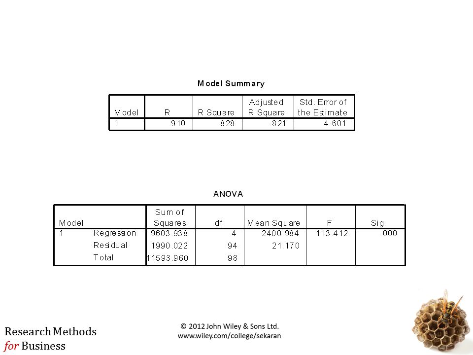
19. Model Significance H1: Not H0
H0: 0 = 1 = ... = m = 0 (all parameters are zero)
H1: Not H0

20. Model Significance
H0: 0 = 1 = ... = m = 0 (all parameters are zero)
H1: Not H0
Test statistic (k = # of variables excl. intercept)
F = (SSReg/k) ~ Fk, n-1-k
(SSe/(n – 1 – k)
SSReg = explained variation by regression
SSe = unexplained variation by regression

21. SPSS

22. Parameter significance
Testing that a specific parameter is significant (i.e., j  0)
H0: j = 0
H1: j  0
Test-statistic: t = bj/SEj ~ tn-k-1
with bj = the estimated coefficient for j
SEj = the standard error of bj

23. SPSS cont’d

24. Physical Attractiveness
Conceptual Model +
Likelihood
to Date
Physical Attractiveness

25. Multiple Regression Analysis
We use more than one (metric or non-metric) independent variable to explain variance in a (metric) dependent variable.

26. Conceptual Model + + Perceived Intelligence Likelihood
to Date
Physical Attractiveness

28. Conceptual Model + + + Gender Perceived Intelligence Likelihood
to Date
Physical Attractiveness

29. Moderators
Moderator is qualitative (e.g., gender, race, class) or quantitative (e.g., level of reward) that affects the direction and/or strength of the relation between dependent and independent variable
Analytical representation
Y = ß0 + ß1X1 + ß2X2 + ß3X1X with Y = DV X1 = IV X2 = Moderator

31. interaction significant effect on dep. var.

32. Conceptual Model + + + + + Gender Perceived Intelligence Likelihood
to Date
Physical Attractiveness + +
Communality of Interests
Perceived Fit

33. Mediating/intervening variable
Accounts for the relation between the independent and dependent variable
Analytical representation
Y = ß0 + ß1X => ß1 is significant
M = ß2 + ß3X => ß3 is significant
Y = ß4 + ß5X + ß6M => ß5 is not significant => ß6 is significant
With Y = DV
X = IV
M = mediator

34. Step 1

35. significant effect on dep. var.
Step 1 cont’d
significant effect on dep. var.

36. Step 2

37. significant effect on mediator
Step 2 cont’d
significant effect on mediator

38. Step 3

39. Step 3 cont’d insignificant effect of indep. var on dep. Var.
significant effect of mediator on dep. var.