1. Computer Graphics (Fall 2008) COMS 4160, Lecture 18: Illumination and Shading 1 http://www.cs.columbia.edu/~cs4160

2. Rendering: 1960s (visibility)  Roberts (1963), Appel (1967) - hidden-line algorithms  Warnock (1969), Watkins (1970) - hidden-surface  Sutherland (1974) - visibility = sorting Images from FvDFH, Pixar’s Shutterbug Slide ideas for history of Rendering courtesy Marc Levoy

3. 1970s - raster graphics  Gouraud (1971) - diffuse lighting, Phong (1974) - specular lighting  Blinn (1974) - curved surfaces, texture  Catmull (1974) - Z-buffer hidden-surface algorithm Rendering: 1970s (lighting)

4. Rendering (1980s, 90s: Global Illumination) early 1980s - global illumination  Whitted (1980) - ray tracing  Goral, Torrance et al. (1984) radiosity  Kajiya (1986) - the rendering equation

5. Outline  Preliminaries  Basic diffuse and Phong shading  Gouraud, Phong interpolation, smooth shading  Formal reflection equation For today’s lecture, slides and chapter 9 in textbook

6. Motivation  Objects not flat color, perceive shape with appearance  Materials interact with lighting  Compute correct shading pattern based on lighting  This is not the same as shadows (separate topic)  Some of today’s lecture review of last OpenGL lec.  Idea is to discuss illumination, shading independ. OpenGL  Today, initial hacks (1970-1980)  Next lecture: formal notation and physics

7. Linear Relationship of Light  Light energy is simply sum of all contributions  Terms can be calculated separately and later added:  multiple light sources  multiple interactions (diffuse, specular, more later)  multiple colors (R-G-B, or per wavelength)

8. General Considerations Surfaces have a position, and a normal at every point. Other vectors used  L = vector to the light source light position minus surface point position  E = vector to the viewer (eye) viewer position minus surface point position (x 1,y 1,z 1 ) N1N1 (x 2,y 2,z 2 ) N2N2

9. Diffuse Lambertian Term  Rough matte (technically Lambertian) surfaces  Not shiny: matte paint, unfinished wood, paper, …  Light reflects equally in all directions  Obey Lambert’s cosine law  Not exactly obeyed by real materials N -L

10. Meaning of negative dot products  If (N dot L) is negative, then the light is behind the surface, and cannot illuminate it.  If (N dot E) is negative, then the viewer is looking at the underside of the surface and cannot see it’s front-face.  In both cases, I is clamped to Zero.

11. Phong Illumination Model  Specular or glossy materials: highlights  Polished floors, glossy paint, whiteboards  For plastics highlight is color of light source (not object)  For metals, highlight depends on surface color  Really, (blurred) reflections of light source Roughness

12. Idea of Phong Illumination  Find a simple way to create highlights that are view- dependent and happen at about the right place  Not physically based  Use dot product (cosine) of eye and reflection of light direction about surface normal  Alternatively, dot product of half angle and normal  Raise cosine lobe to some power to control sharpness

13. Phong Formula -L R E

14. Alternative: Half-Angle (Blinn-Phong)  In practice, both diffuse and specular components H N

15. Outline  Preliminaries  Basic diffuse and Phong shading  Gouraud, Phong interpolation, smooth shading  Formal reflection equation Not in text. If interested, look at FvDFH pp 736-738

16. Triangle Meshes as Approximations  Most geometric models large collections of triangles.  Triangles have 3 vertices with position, color, normal  Triangles are approximation to actual object surface

17. Vertex Shading  We know how to calculate the light intensity given:  surface position  normal  viewer position  light source position (or direction)  2 ways for a vertex to get its normal:  given when the vertex is defined  take normals from faces that share vertex, and average

18. Coloring Inside the Polygon  How do we shade a triangle between it’s vertices, where we aren’t given the normal?  Inter-vertex interpolation can be done in object space (along the face), but it is simpler to do it in image space (along the screen).

19. Flat vs. Gouraud Shading Flat - Determine that each face has a single normal, and color the entire face a single value, based on that normal. Gouraud – Determine the color at each vertex, using the normal at that vertex, and interpolate linearly for the pixels between the vertex locations. glShadeModel(GL_FLAT)glShadeModel(GL_SMOOTH)

20. Gouraud Shading – Details Scan line Actual implementation efficient: difference equations while scan converting

21. Gouraud and Errors  I 1 = 0 because (N dot E) is negative.  I 2 = 0 because (N dot L) is negative.  Any interpolation of I 1 and I 2 will be 0. I 1 = 0I 2 = 0 area of desired highlight

22. 2 Phongs make a Highlight  Besides the Phong Reflectance model (cos n ), there is a Phong Shading model.  Phong Shading: Instead of interpolating the intensities between vertices, interpolate the normals.  The entire lighting calculation is performed for each pixel, based on the interpolated normal. (OpenGL doesn’t do this, but you can with current programmable shaders) I 1 = 0I 2 = 0

23. Problems with Interpolated Shading  Silhouettes are still polygonal  Interpolation in screen, not object space: perspective distortion  Not rotation or orientation-independent  How to compute vertex normals for sharply curving surfaces?  But at end of day, polygons are mostly preferred to explicitly representing curved objects like spline patches for rendering

24. Outline  Preliminaries  Basic diffuse and Phong shading  Gouraud, Phong interpolation, smooth shading  Formal reflection equation

25. Motivation Lots of ad-hoc tricks for shading –Kind of looks right, but? Physics of light transport –Will lead to formal reflection equation One of the more formal lectures –But important to solidify theoretical framework

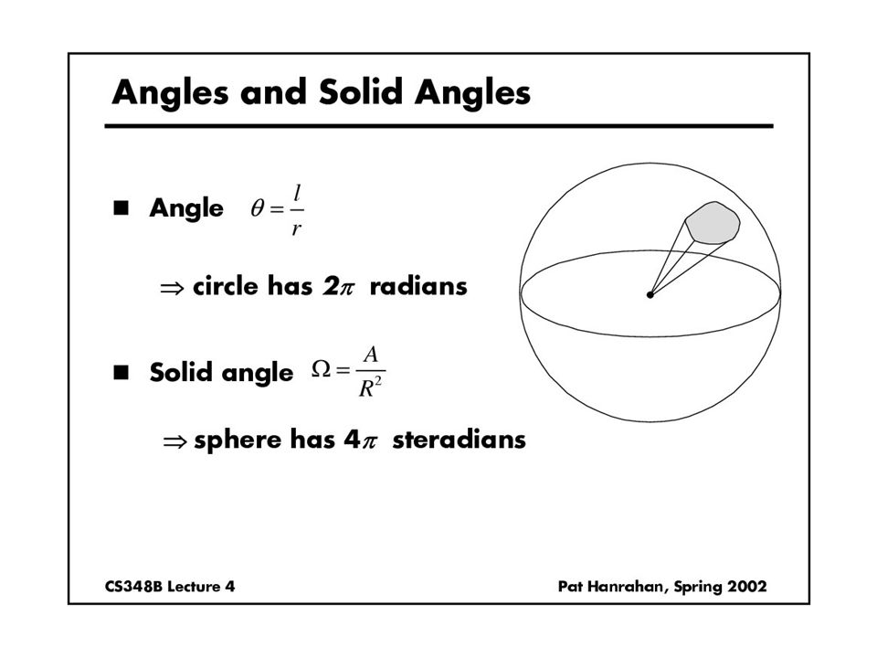
29. Radiance Power per unit projected area perpendicular to the ray per unit solid angle in the direction of the ray Symbol: L(x,ω) (W/m 2 sr) Flux given by dΦ = L(x,ω) cos θ dω dA

30. Radiance properties Radiance is constant as it propagates along ray –Derived from conservation of flux –Fundamental in Light Transport.

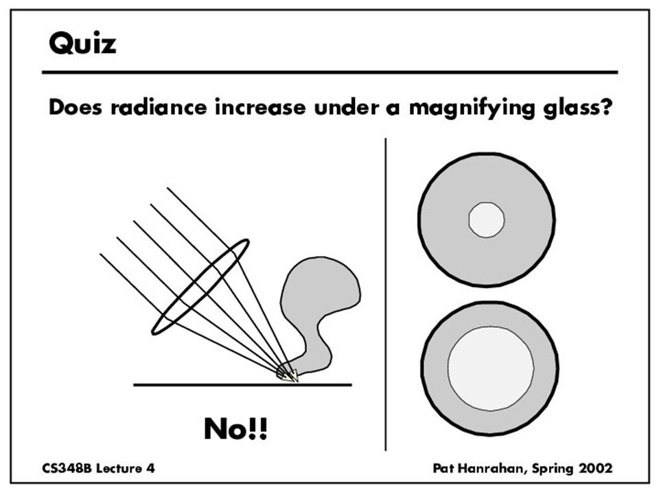
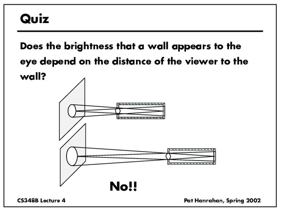
33. Radiance properties Sensor response proportional to radiance (constant of proportionality is throughput) –Far away surface: See more, but subtends smaller angle –Wall equally bright across viewing distances Consequences –Radiance associated with rays in a ray tracer –Other radiometric quants derived from radiance

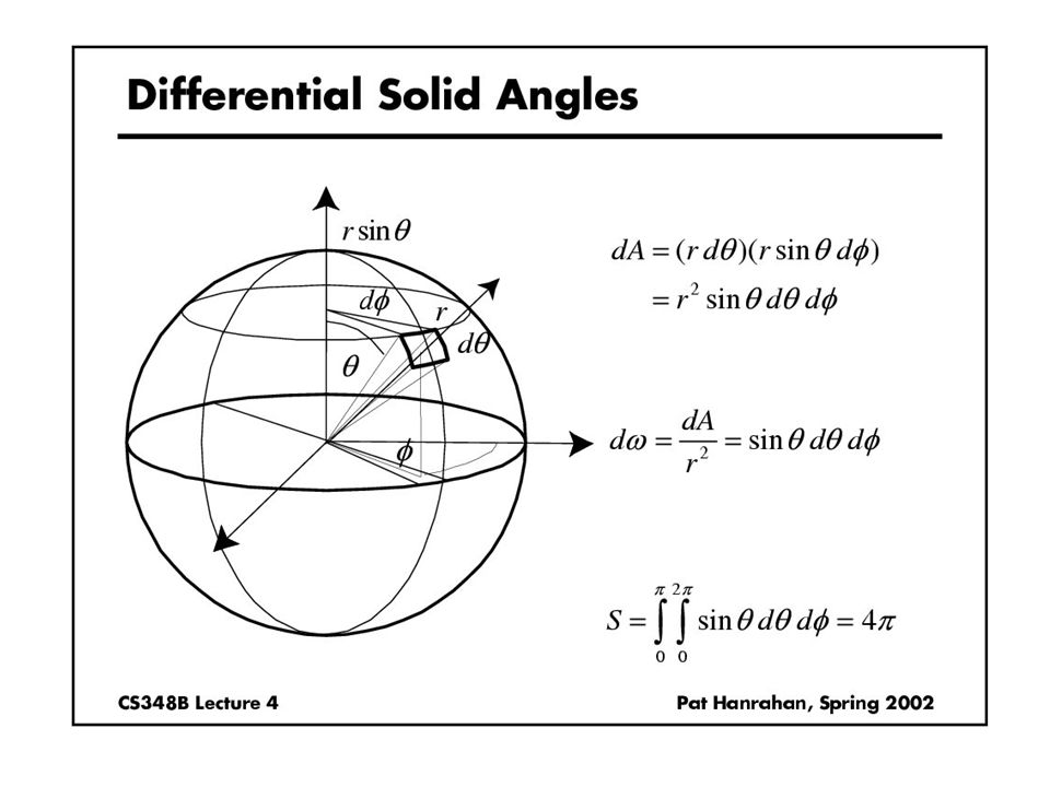
34. Irradiance, Radiosity Irradiance E is radiant power per unit area Integrate incoming radiance over hemisphere –Projected solid angle (cos θ dω) –Uniform illumination: Irradiance = π [CW 24,25] –Units: W/m 2 Radiosity –Power per unit area leaving surface (like irradiance)

35. Building up the BRDF Bi-Directional Reflectance Distribution Function [Nicodemus 77] Function based on incident, view direction Relates incoming light energy to outgoing light energy We have already seen special cases: Lambertian, Phong In this lecture, we study all this abstractly

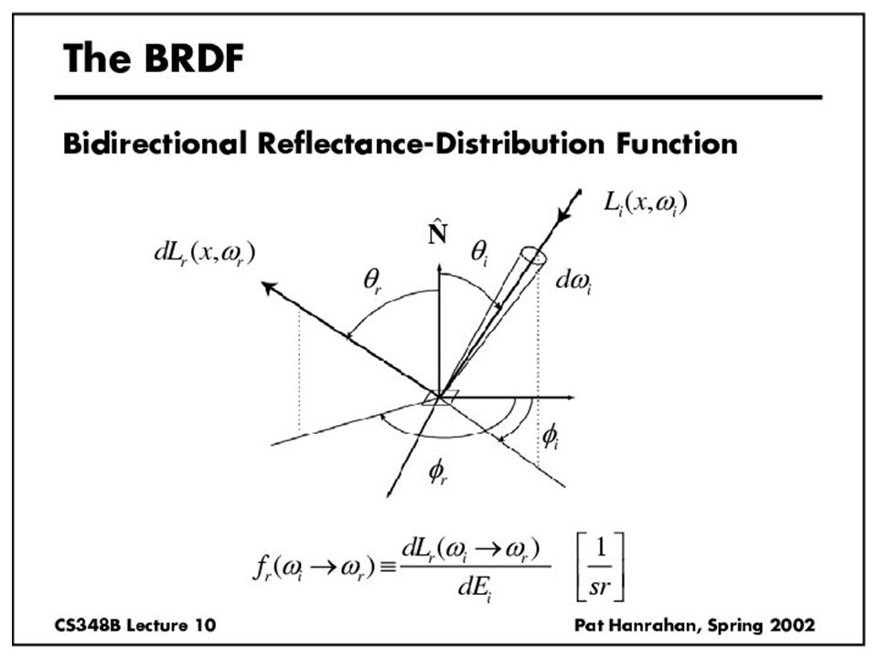
37. BRDF Reflected Radiance proportional to Irradiance Constant proportionality: BRDF [CW pp 28,29] –Ratio of outgoing light (radiance) to incoming light (irradiance) –Bidirectional Reflection Distribution Function –(4 Vars) units 1/sr

38. Reflection Equation Reflected Radiance (Output Image) Incident radiance (from light source) BRDF Cosine of Incident angle

39. Reflection Equation Sum over all light sources Reflected Radiance (Output Image) Incident radiance (from light source) BRDF Cosine of Incident angle

40. Reflection Equation Replace sum with integral Reflected Radiance (Output Image) Incident radiance (from light source) BRDF Cosine of Incident angle