Download presentation
Presentation is loading. Please wait.

1
Regresión Lineal Simple PlantaCapVol Rosario25567.65 Coyoacán4005676.48 Acueducto de Guadalupe871923.7 San Juan de Aragón5004446.58 Ciudad Deportiva2304099.68 Iztacalco13315.36 Cerro de la Estrella400046957.1 San Pedro Atocpan601103.76 San Juan Ixtayopan15252.29 San Andrés Mixquic30946.08 Abasolo15157.68 Heroico Colegio Militar30630.72 Parres731.54 PEMEX26315.36 Xicalco794.6 Reclusorio Sur30378.43 San Luis Tlaxialtemalco1501892.16 Tlatelolco22378.43 Bosque de las Lomas55473.04 Campo Militar No. 130378.43 Chapultepec1602018.3 RS1. Plantas de Tratamiento de agua, DF, 1998

2
anova(modelo) Analysis of Variance Table Response: Vol Df Sum Sq Mean Sq F value Pr(>F) Cap12029113094 2029113094 6676.1 < 2.2e-16 *** Residuals195774809303937 Total202034887903 --- Signif. codes: 0 ‘***’ 0.001 ‘**’ 0.01 ‘*’ 0.05 ‘.’ 0.1 ‘ ’ 1 summary(modelo) Call: lm(formula = Vol ~ Cap) Residuals: Min1Q Median3QMax -1593.94-188.53-60.9678.991212.30 Coefficients: EstimateStd. Errort valuePr(>|t|) (Intercept)201.3821126.81221.5880.129 Cap11.67830.142981.707<2e-16 *** --- Signif. codes: 0 ‘***’ 0.001 ‘**’ 0.01 ‘*’ 0.05 ‘.’ 0.1 ‘ ’ 1 Residual standard error: 551.3 on 19 degrees of freedom Multiple R-squared: 0.9972, Adjusted R-squared: 0.997 F-statistic: 6676 on 1 and 19 DF, p-value: < 2.2e-16
 Call: lm(formula = Vol ~ Cap) Residuals: Min1Q Median3QMax Coefficients: EstimateStd. Errort valuePr(>|t|) (Intercept) Cap <2e-16 *** --- Signif. codes: 0 ‘***’ ‘**’ 0.01 ‘*’ 0.05 ‘.’ 0.1 ‘ ’ 1 Residual standard error: on 19 degrees of freedom Multiple R-squared: , Adjusted R-squared: F-statistic: 6676 on 1 and 19 DF, p-value: < 2.2e-16.")
3
shapiro.test(modelo$residual) Shapiro-Wilk normality test data: modelo$residual W = 0.8475, p-value =0.003846
 Shapiro-Wilk normality test data: modelo$residual W = , p-value =")
4
Transformación de variable y<-sqrt(Vol) m2<-lm(y~Cap) Analysis of Variance Table Response: y Df Sum Sq Mean Sq F value Pr(>F) Cap 1 36673 36673 184.94 3.047e-11 *** Residuals 193768198 --- Signif. codes: 0 ‘***’ 0.001 ‘**’ 0.01 ‘*’ 0.05 ‘.’ 0.1 ‘ ’ 1 Shapiro-Wilk normality test data: m2$residuals W = 0.9196, p-value = 0.08506

5
RS2. Modelo de Pinzones summary(m) Call: lm(formula = beak.length ~ mass, data = KenyaFinches) Residuals: Min1QMedian3QMax -1.05373 -0.27044 -0.05373 0.33806 0.82956 Coefficients: Estimate Std. Error t value Pr(>|t|) (Intercept) 6.487159 0.112906 57.46 <2e-16 *** mass 0.110411 0.004608 23.96 <2e-16 *** --- Signif. codes: 0 ‘***’ 0.001 ‘**’ 0.01 ‘*’ 0.05 ‘.’ 0.1 ‘ ’ 1 Residual standard error: 0.4174 on 43 degrees of freedom Multiple R-squared: 0.9303, Adjusted R-squared: 0.9287 F-statistic: 574 on 1 and 43 DF, p-value: Schluter, D. 1988. The evolution of finch communities on islands and continents: Kenya vs. Galapagos. Ecological Monographs 58: 229-249.
 Call: lm(formula = beak.length ~ mass, data = KenyaFinches) Residuals: Min1QMedian3QMax Coefficients: Estimate Std. Error t value Pr(>|t|) (Intercept) <2e-16 *** mass <2e-16 *** --- Signif. codes: 0 ‘***’ ‘**’ 0.01 ‘*’ 0.05 ‘.’ 0.1 ‘ ’ 1 Residual standard error: on 43 degrees of freedom Multiple R-squared: , Adjusted R-squared: F-statistic: 574 on 1 and 43 DF, p-value: Schluter, D The evolution of finch communities on islands and continents: Kenya vs. Galapagos. Ecological Monographs 58:")
6
anova(m) Analysis of Variance Table Response: beak.length DfSum SqMean SqFvalue Pr(>F) Mass1100.000100.000574.03< 2.2e-16 *** Residuals 43 7.491 0.174 Total44107.491 --- Signif. codes: 0 ‘***’ 0.001 ‘**’ 0.01 ‘*’ 0.05 ‘.’ 0.1 ‘ ’ 1 shapiro.test(m$residuals) Shapiro-Wilk normality test data: m$residuals W = 0.9784, p-value = 0.5572
 Shapiro-Wilk normality test data: m$residuals W = , p-value =")
7
RS3. Reforestación en el DF m<-lm(Reforestacion~Superfice) summary(m) Call: lm(formula = Reforestacion ~ Superfice) Residuals: Min 1Q Median 3Q Max -148.43 -97.75 -10.08 92.44 180.59 Coefficients: Estimate Std. Error t value Pr(>|t|) (Intercept)186.380142.25764.4110.000593 *** Superfice-0.30780.3439-0.8950.385911 --- Signif. codes: 0 ‘***’ 0.001 ‘**’ 0.01 ‘*’ 0.05 ‘.’ 0.1 ‘ ’ 1 Residual standard error: 111.4 on 14 degrees of freedom Multiple R-squared: 0.05412, Adjusted R-squared: -0.01344 F-statistic: 0.801 on 1 and 14 DF, p-value: 0.3859
 summary(m) Call: lm(formula = Reforestacion ~ Superfice) Residuals: Min 1Q Median 3Q Max Coefficients: Estimate Std. Error t value Pr(>|t|) (Intercept) *** Superfice Signif. codes: 0 ‘***’ ‘**’ 0.01 ‘*’ 0.05 ‘.’ 0.1 ‘ ’ 1 Residual standard error: on 14 degrees of freedom Multiple R-squared: , Adjusted R-squared: F-statistic: on 1 and 14 DF, p-value:")
8
anova(m) Analysis of Variance Table Response: Reforestacion Df Sum SqMean SqF valuePr(>F) Superfice199439943.10.8010.3859 Residuals1417377812412.7 Total15183721
 Analysis of Variance Table Response: Reforestacion Df Sum SqMean SqF valuePr(>F) Superfice Residuals Total")
10
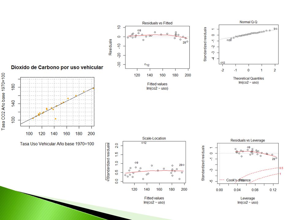
RS4. Dióxido de Carbono por uso vehicular anioco2uso 1971104.619105.742 1972109.785110.995 1973117.197116.742 1974114.404114.592 1975111.994115.605 1976116.898121.467 1977119.915123.123 1978126.07127.953 1979128.759127.648 1980130.196135.66 1981126.409138.139 1982103.136141.911 1983134.212143.707 1984140.721151.205 1985143.462154.487 1986153.074162.285 1987159.999174.837 1988170.312187.403 1989177.51202.985 1990182.686204.959 1991181.348205.325 1992183.757205.598 1993185.869205.641 1994186.872210.826 1995185.1214.947 1996192.249220.753 1997194.667225.742 1998193.438229.027 Año base 1970=100 Redfern, A., Bunyan, M., and Lawrence, T. (eds) (2003). The Environment in Your Pocket, 7 th edn. London: UK Department for Environment, Food and Rural Affairs.
 (2003). The Environment in Your Pocket, 7 th edn. London: UK Department for Environment, Food and Rural Affairs..")
11
Call: lm(formula = co2 ~ uso) Residuals: Min 1Q Median 3Q Max -29.5946 -0.7761 1.0901 2.4873 6.8163 Coefficients: Estimate Std. Error t value Pr(>|t|) (Intercept) 25.39475 5.05584 5.023 3.16e-05 *** uso 0.75636 0.02999 25.223 < 2e-16 *** --- Signif. codes: 0 ‘***’ 0.001 ‘**’ 0.01 ‘*’ 0.05 ‘.’ 0.1 ‘ ’ 1 Residual standard error: 6.503 on 26 degrees of freedom Multiple R-squared: 0.9607, Adjusted R-squared: 0.9592 F-statistic: 636.2 on 1 and 26 DF, p-value: < 2.2e-16 Analysis of Variance Table Response: co2 DfSum SqMean SqFvalue Pr(>F) Uso126904.126904.1 636.21 < 2.2e-16 *** Residuals 26 1099.5 42.3 Total2728003.6 --- Signif. codes: 0 ‘***’ 0.001 ‘**’ 0.01 ‘*’ 0.05 ‘.’ 0.1 ‘ ’ 1
 (Intercept) e-05 *** uso < 2e-16 *** --- Signif. codes: 0 ‘***’ ‘**’ 0.01 ‘*’ 0.05 ‘.’ 0.1 ‘ ’ 1 Residual standard error: on 26 degrees of freedom Multiple R-squared: , Adjusted R-squared: F-statistic: on 1 and 26 DF, p-value: < 2.2e-16 Analysis of Variance Table Response: co2 DfSum SqMean SqFvalue Pr(>F) Uso < 2.2e-16 *** Residuals Total Signif. codes: 0 ‘***’ ‘**’ 0.01 ‘*’ 0.05 ‘.’ 0.1 ‘ ’ 1.")
Similar presentations

 Coefficients of Determination BMTRY 701 Biostatistical Methods II.>")


![x y z The data as seen in R [1,] 58035 354.559 46 population city manager compensation [2,] 120100 351.593 998 [3,] 102743 339.815 615 [4,] 117242 321.533.](/16/4932610/big_thumb.jpg "x y z The data as seen in R [1,] 58035 354.559 46 population city manager compensation [2,] 120100 351.593 998 [3,] 102743 339.815 615 [4,] 117242 321.533.>")


 variable - measures the outcome of a study. Explanatory (Independent) variable - explains.>")


![Crime? FBI records violent crime, z x y z [1,] 58035 354.559 46 [2,] 120100 351.593 998 [3,] 102743 339.815 615 [4,] 117242 321.533 168 [5,] 137538.](/17/5355243/big_thumb.jpg "Crime? FBI records violent crime, z x y z [1,] 58035 354.559 46 [2,] 120100 351.593 998 [3,] 102743 339.815 615 [4,] 117242 321.533 168 [5,] 137538.>")