1. Population Genetics Kellet’s whelk Kelletia kelletii mtDNA COI & 11 microsatellite markers 28 sampling sites across entire range 1000+ larvae in each capsule

2. P = 0.1

4. Prominent barriers to gene flow Point Conception Punta Eugenia

5. Point Conception

6. 100 km Point Conception Punta Eugenia Expanded range High genetic diversity

7. 100 km Genetic isolation by geographic distance Estimated mean dispersal distance in 10s of km 100 km Geographic distance Point Conception Punta Eugenia Genetic difference Expanded range High genetic diversity

8. 100 km Genetic isolation by geographic distance Estimated mean dispersal distance in 10s of km 100 km Geographic distance Point Conception Punta Eugenia Genetic difference Expanded range High genetic diversity

9. Geographic distance Genetic difference

10. Oceanographic connectivity Genetic difference

11. Lagrangian Particle Trajectories Velocity fields from Oey et al. [2003] data assimilation

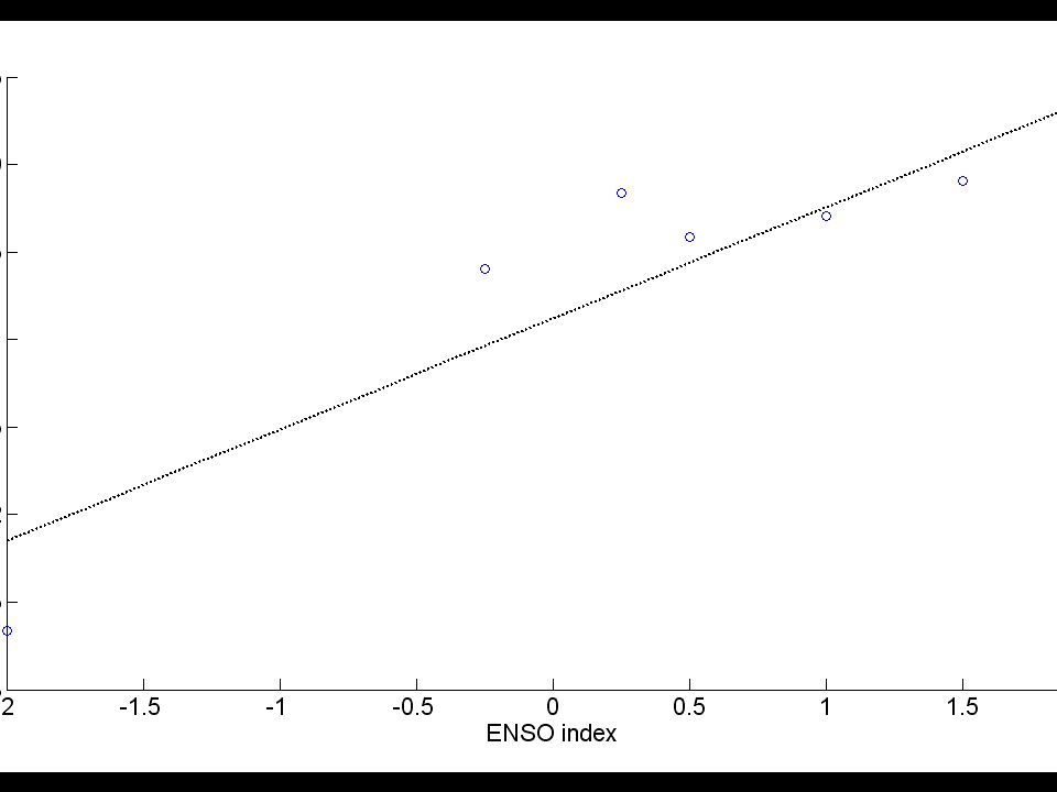
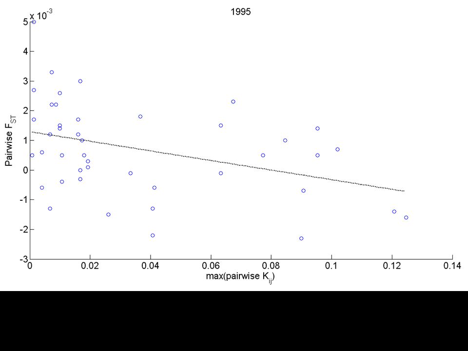
12. P = 0.006 (Mantel test) 1995

13. Negative ENSO (i.e., la Nina) oceanographic conditions correlate most strongly with predicted pattern of gene flow P = 0.009 (all years) P = 0.078 (remove 1999)

14. Negative ENSO (i.e., la Nina) oceanographic conditions correlate most strongly with predicted pattern of gene flow All P-values calculated via Mantel Test (10,000 permutations) P = 0.3 0.15 0.006 0.024 0.071 0.027 0.039 P = 0.009 (all years) P = 0.078 (remove 1999)

15. P = 0.009 (all years) P = 0.078 (remove 1999)

16. Vorticity “Effective dispersal” may predominantly occur during la Nina conditions

17. Are reserves good for fisheries?

18. Oikos 2007 Spatially-implicit difference equations:

19. Reserves enhance fishery yield (White and Kendall 2007 Oikos)

20. Fishing costs money

21. Reserves still enhance fishery profit

22. POPULATION REGULATION Density dependent larval recruitment  Inter-cohort: Adults compete with larvae for space and food as they grow older  Intra-cohort: Larvae compete amongst themselves for space and food

23. Spatially and Temporally Explicit Integrodifference Model Settlers at x = R = proportion of settlers that successfully recruit into the local population

24. Spatially and Temporally Explicit Integrodifference Model Ricker: Density dependence:Inter-cohort Intra-cohort

25. Spatially and Temporally Explicit Integrodifference Model Beverton-Holt: Density dependence:Inter-cohort Intra-cohort

26. Hastings & Botsford 1999 Gaylord et al. 2005 White & Kendall 2007 White et al. In Review Ecol Lett Increasing cost of fishing Density dependence Inter-cohort Intra-cohort Reserves do not necessarily enhance fishery profit Gray horizontal plane represents equivalence Costello & Ward In Prep.

27. Optimal management Impractical to implement / regulate

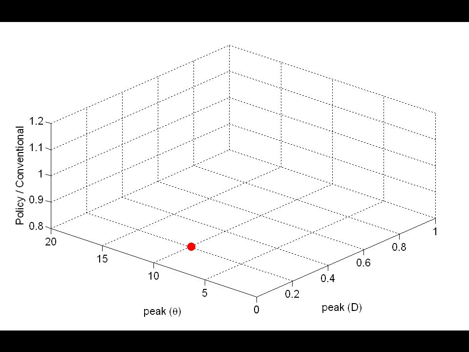
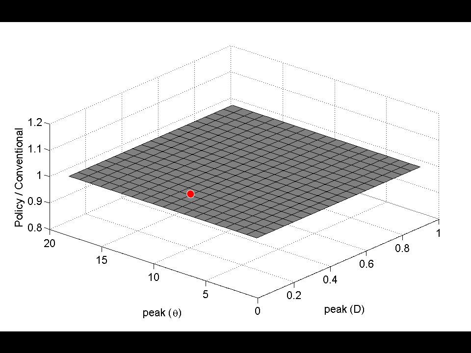
28. For reserves to work, policy must have a single %MPA regulated across the entire fishing community (“Community MPA”). Note: escapement can still be species-specific Question: Given a community of fishery species in a region characterized by a set of D- and θ-values, does “Community MPA” management enhance profit compared to conventional management?

30. Cod Wrasse Cabezon Marine bass RockfishScallop Lobster Urchin & damselfish Kelp Coral

31. Example community distribution

33. Sub-sampling of evaluated β distributions All distributions with peak(D) = 0.2 All distributions with peak(θ) = 10

34. Sub-sampling of evaluated β distributions

35. Evaluated β distributions

36. Sub-sampling of evaluated β distributions All distributions with peak(D) = 0.2 All distributions with peak(θ) = 10

37. Each point represents the mean of all species assemblage distributions with same peak

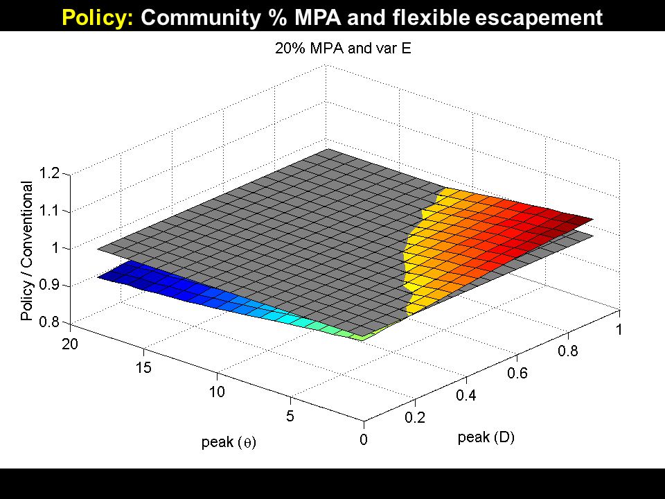
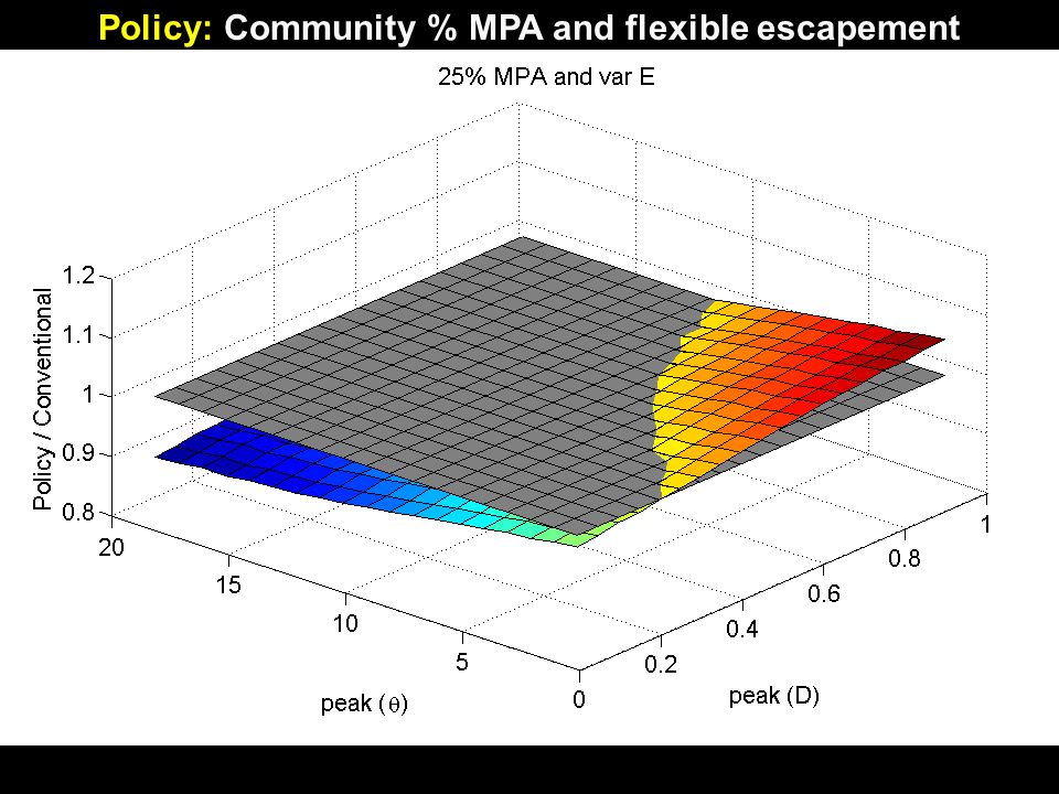
40. Policy: Community % MPA and flexible escapement

50. Large % MPA is a poor policy, unless confident θ 0.6 Consequences of miscalculation are severe Policy: Community % MPA and flexible escapement

51. Moderate % MPA is a decent compromise policy, Consequences of miscalculation are not severe Max 10% loss Policy: Community % MPA and flexible escapement

52. Conclusions (part I): Choosing a policy  Optimal management is impractical because depends on species- specific %MPAs  Optimal Community %MPA depends on θ and D  Cheap, inter-cohort species dominate fishery → Reserves good  Expensive, intra-cohort species dominate fishery → Reserves bad  Given zero knowledge of θ or D, conventional management is least risky option  Common scenario: 20% MPA  Okay compromise. Worst-case negative consequences generate 90% profits compared to optimal conventional management

53. Question: Given a Community %MPA policy what is optimal escapement? Note: includes %MPA = 0 Are there rules of thumb?

54. Optimal escapement, given… Harvest all fish

55. Optimal escapement, given… Minimal variance across D-values Harvest all fish

56. Optimal escapement, given… Harvest all fish

57. Optimal escapement, given… Harvest all fish

58. Optimal escapement, given… Harvest all fish

59. Optimal escapement, given… Harvest all fish

60. Optimal escapement, given… Harvest all fish

61. Dependent variable: Optimal escapement Independent variableR square D < 0.005 θ 0.70 %MPA 0.23 θ & %MPA 0.94 Multiple Linear Regression

62. Dependent variable: Optimal escapement Independent variableR square Model (BH or Ricker) 2e-5 P (fecundity) 0.05 m (mortality) 0.01 D < 0.01 θ 0.62 %MPA 0.19 θ & %MPA 0.81 Multiple Linear Regression

63. Escapement = 0.014* θ – 0.30*(%MPA) + 0.18 R square = 0.81 P < 1e-10

64. Optimal management Ricker P = 1 m = 0.1

65. Policy: P1 = Optimal management When reserves are part of optimal solution

66. Conclusions (part II): Policy regulation  Optimal escapement decreases as % MPA increases  Fish harder to make up for displacement by reserves  Given community % MPA policy  Escapement decreases with decreasing cost of fishing (θ → 0)  The cheaper the fishing, the harder you should fish  Escapement minimally influenced by D, m, P or model form  Once a policy is implemented (whether conventional or with reserves):  Avoid spending time/money/effort estimating demographic profiles for each fishery species  Focus on developing efficient method for regulating escapement in relation to θ (e.g., via a tax)

75. Fishing costs money

76. Negative ENSO (i.e., la Nina) oceanographic conditions correlate most strongly with predicted pattern of gene flow All correlations significant (P < 0.05; Mantel) except 1997 (strongest el Nino year in record)

78. Pre-harvest Cost Post- harvest θ Population density =

79. M = 0.05 (dash) M = 0.1 (solid) P = 1, 2, 3 (White et al. In Review Ecol Lett) Increasing cost of fishing

80. SOUTHERN CALIFORNIA BIGHT

81. Reserve Radius of larval export from reserve

82. FISHERY PROFIT UNDER OPTIMAL RESERVE VS. CONVENTIONAL MANAGEMENT Ricker P = 1 m = 0.1 Increasing cost of fishing Inter-cohort Intra-cohort Density dependence

83. An integro-difference model describing coastal fish population dynamics: Adult abundance at location x during time-step t+1 Number of adults harvested Natural mortality of adults that escaped being harvested Fecundity Larval survival Larval dispersal (Gaussian) (Siegel et al. 2003) Larval recruitment at x Number of larvae that successfully recruit to location x (White et al. In Review Ecol Lett)

84. Major questions in marine ecology and fisheries management  What is the optimal management strategy for coastal fisheries?  Are reserves a part of the optimal strategy?  How are populations regulated (i.e., where/how does density dependence occur)?  What are the management consequences to different forms of demographic regulation?  How connected are populations?  What drives connectivity, and how variable are patterns of connectivity over time?  What are the management consequences of population connectivity? THESE QUESTIONS APPLY TO ALL RENEWABLE NATURAL RESOURCE MANAGEMENT SCENARIOS

85. Major questions in marine ecology and fisheries management  What is the optimal management strategy for coastal fisheries?  Are reserves a part of the optimal strategy?  How are populations regulated (i.e., where/how does density dependence occur)?  What are the management consequences to different forms of demographic regulation?  How connected are populations?  What drives connectivity, and how variable are patterns of connectivity over time?  What are the management consequences of population connectivity? THESE QUESTIONS APPLY TO ALL RENEWABLE NATURAL RESOURCE MANAGEMENT SCENARIOS

87. “Garibaldi” California Department of Fish and Game

89. Genetic isolation by geographic distance Estimated mean dispersal distance in 10s of km 100 km Geographic distance Genetic difference Point Conception Punta Eugenia 100 km

90. Genetic isolation by geographic distance Estimated mean dispersal distance in 10s of km 100 km Geographic distance Point Conception Punta Eugenia Genetic difference

91. Point Conception Punta Eugenia Expanded range High genetic diversity

92. Point Conception Punta Eugenia Expanded range High genetic diversity

166. (Halpern 2003, Palumbi 2003) Reserves are good for marine life:

168. Focus of developing fishery Sold to US domestic Asian market (mostly in LA) Mean price = $1.43/kg = ~$0.15/whelk Aseltine-Neilson et al. 2006

169. Population and fishery dynamics outside reserves: Population dynamics inside reserves: Questions:  What is the optimal value for c?  If c* > 0, how much better are reserves compared to conventional management? (White and Kendall 2007 Oikos)

170. Optimal Reserves (30 day larval dispersal period) Reserve

171. PROFIT = Pre-harvest Fishery yield at location x during time step t Revenue - Cost Post- harvest

172. Conventional Isolation-by-Distance