Download presentation
Presentation is loading. Please wait.

3
We are focusing our discussion within the luminance dimension. Note, however, that these discussions could also be directed towards the chromatic and/or temporal dimensions as well.

4
Luminance contrastincreasedecrease

5
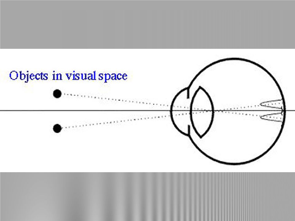
How do images relate to objects in visual space? Properties of the visual SYSTEM.

8
luminance Line Spread Function

13
NOTE: We only recognize the two object lines if the detectors under the image are projecting as separate lines.

14
Linear Systems Analysis - we’re interested in examining the relationship between object intensities and the perceptual representation of those intensities..

15
Optical System Intensity difference input Intensity difference output

16
Lens forming an image of a periodic grating. Modulation Transfer Functions

17
Optical System Intensity input Intensity output Eye is an optical system Intensity output is the retinal image

18
Further sampling error

19
Optical System Intensity input perceptual output Neural System

20
V in (x-axis) V out (y-axis) output signal input signal
 V out (y-axis) output signal input signal")
23
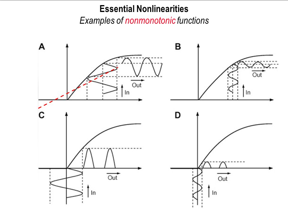
Essential Nonlinearities Examples of nonmonotonic functions

24
Start with the retina..

25
Can we develop a relationship between the screen & retinal image?

26
1. Principle of Homogeneity (intensity distribution). 1. Principle of Superposition (positional distribution). Need to first discuss two basic principles of linearity:
. Need to first discuss two basic principles of linearity:.")
27
p is a vector that represents different positional intensities across the one-dimensional monitor image. Row vector: p=(0.0, 0.0, 1.0, 0.0, 0.0) r is the retinal image vector: r=(0.0, 0.05, 0.55, 0.05, 0.0) r=(0.0, 0.05, 0.55, 0.05, 0.0)
 r is the retinal image vector: r=(0.0, 0.05, 0.55, 0.05, 0.0) r=(0.0, 0.05, 0.55, 0.05, 0.0).")
28
r is the retinal image vector: r=(0.07, 0.65, 0.07, 0.0, 0.0) r=(0.07, 0.65, 0.07, 0.0, 0.0) r is the retinal image vector: r=(0.00, 0.00, 0.07, 0.65, 0.07) r=(0.00, 0.00, 0.07, 0.65, 0.07) p is a vector that represents different positional intensities across the one-dimensional monitor image. Row vector: p=(0.0, 1.0, 0.0, 0.0, 0.0) p=(0.0, 0.0, 0.0, 1.0, 0.0) p=(0.0, 1.0, 0.0, 1.0, 0.0) r is the retinal image vector: r=(0.07, 0.65, 0.45, 0.65, 0.07) r=(0.07, 0.65, 0.45, 0.65, 0.07)
 p=(0.0, 0.0, 0.0, 1.0, 0.0) p=(0.0, 1.0, 0.0, 1.0, 0.0) r is the retinal image vector: r=(0.07, 0.65, 0.45, 0.65, 0.07) r=(0.07, 0.65, 0.45, 0.65, 0.07).")
29
Designate the scalars

30
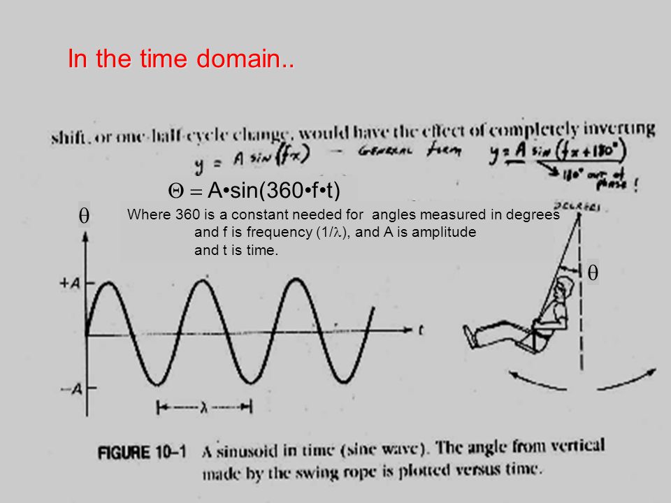
Again, define spatial frequency.. First start with sine wave functions w/ time

32
Asin(360ft) Where 360 is a constant needed for angles measured in degrees and f is frequency (1/ ), and A is amplitude and t is time. In the time domain..

33
Spatial frequency is defined as so many cycles per 1° visual angle (cpd or cyc/deg). Position (or Spatial Extent)
.")
36
Michelson Contrast defines contrast for periodic patterns.

37
NOTE: Aperiodic Contrast is usually defined as the % difference between object & background luminance.

40
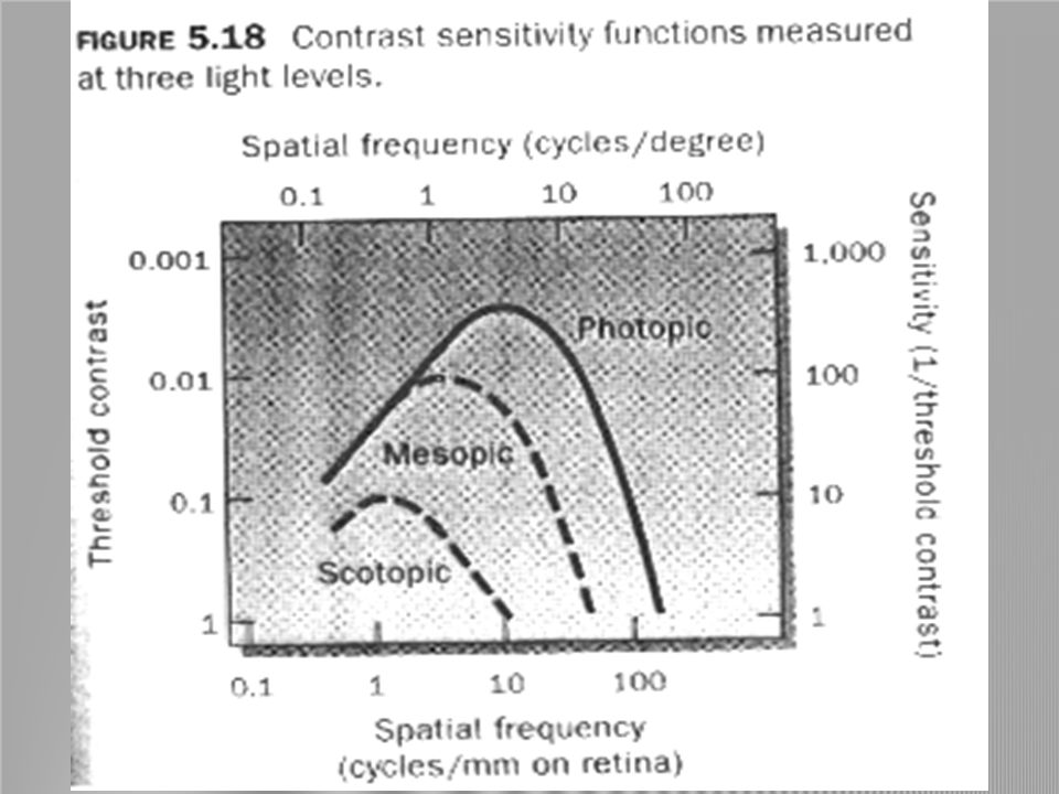
Grating sensitivity Grating sensitivity, as measured in psychophysical threshold experiments. The left-hand graph shows the luminance contrast required to detect the presence of a grating, as a function of its spatial frequency and mean luminance. The subject requires least contrast to detect gratings at medium spatial frequencies. The right-hand graph re-plots the data in terms of contrast sensitivity (1/contrast) as a function of spatial frequency. Data are taken from Campbell and Robson (1968).
 as a function of spatial frequency. Data are taken from Campbell and Robson (1968)..")
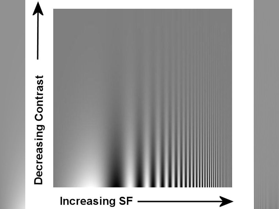
43
Note: Different appearing contrasts for different spatial frequencies.

46
Spatial frequency

47
Mouse “GO/NO GO” determination of 90° orientation sensitivity with and without optogenetically activated cholinergic basal forebrain modulation of V1.

48
Normal Amblyopia MS Cataract

50
To determine the modulation transfer function MTF of an optical system, you need to compare the magnitude of image contrast with that of the object contrast. This defines the spatial filtering properties of the system (amplitude energy loss through the system).
..")
51
Comparing image contrast to object contrast.

53
Common Optical MTFs c/deg or cpd in vision

54
What is amplitude energy loss? First: The spatial energy of an image is defined by the component sine waves and their component amplitudes.

55
If two sine-wave gratings of different frequencies are superimposed upon each other, the resulting pattern of illumination can be found by adding the two sine waves together, point by point.

57
This means you can combine different spatial frequencies to create a compound image..

58
++ Lower contrastFundamentals

60
Continue the summation process with higher and higher spatial frequencies of proportionally lower & lower amplitudes..

62
Now is as good a time as any to note the difference between a square-wave and sine- wave grating..

63
This is the square wave’s fundamental frequency

64
Note: By adding together sine waves of various frequencies, amplitudes & orientations, it is possible to obtain distributions of many different shapes.

66
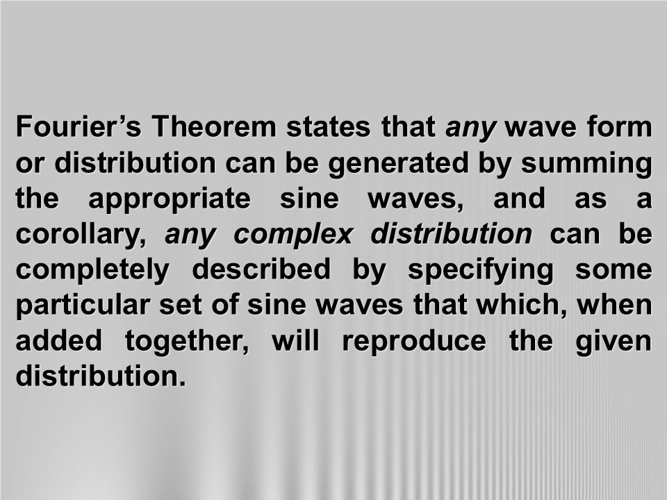
Fourier’s Theorem states that any wave form or distribution can be generated by summing the appropriate sine waves, and as a corollary, any complex distribution can be completely described by specifying some particular set of sine waves that which, when added together, will reproduce the given distribution.

67
The procedure for finding the particular set of sine waves that must be added in order to obtain some given complex waveform is called Fourier analysis. The sine wave components are the Fourier components of a complex wave. Each Fourier component has its own contributing amplitude (or energy state).
..")
68
Now, back to the original question: What is amplitude energy loss? The spatial energy of an image is defined by its component sine waves and the component amplitudes. Specific energy can be characterized by the spatial spectrum (Energy as a function of Spatial Frequency)..
...")
69
Spatial Spectrum: Amplitude as a function of spatial frequency.

70
Spatial scale and spatial frequency 1 [ Summation of 1-D spatial frequency components to create complex spatial waveforms. As a series of components are added progressively to the waveform, the resultant image approximates a square wave more closely.

73
Do a Fourier analysis to get spatial spectrum. Amplitude of modulation of object Modulation of image relative to object Amplitude of modulation of image Spatial Frequency cycles/inch MTF Filtered result:

74
F F -1 Parts of the spectrum are continuous because all the spatial frequencies are included in the object.

75
Note: Spatial spectra DO NOT represent position. They only represent the periodic energy content of the complex image across one dimension. E E f f f

77
Again, these analyses are based on 1-dimensional evaluations. Can have Fourier across multiple dimensions to best represent the components of an image. Also, the multiple dimensional Fourier is not always intuitive (e.g., checkerboard pattern): Energy of the spectrum conforms to 45° distribution with fundamental at the shorter √ 2 distance from edge-to-edge. fundamental
: Energy of the spectrum conforms to 45° distribution with fundamental at the shorter √ 2 distance from edge-to-edge. fundamental.")
78
Human MTF is also the CSF. Includes optical degradation of the eye & neural spatial errors. Position (minutes of arc) Spectrum of Mach Band intensity distribution input Spatial Frequency Spatial Frequency cycles/degree Position (minutes of arc) intensity F -1 F
 Spectrum of Mach Band intensity distribution input Spatial Frequency Spatial Frequency cycles/degree Position (minutes of arc) intensity F -1 F.")
79
The Human MTF (i.e., the CSF) reinforces our perception of edges! This is what, in fact, the brain accomplishes.

80
F -1 F Theoretically, based on MTF analysis, there should be no difference in perceived image.

82
Problem: visual system also operates on the principles of image position as well as amplitude energy -- the latter of which is position irrelevant.

83
In fact, we already know there are spatially linear RFs that make up our visual substrate. So position is relevant. Our cells are not mere Fourier analyzers! Having said this, however, our concept of scale certainly has bearing on spatial frequency.

84
Images contain detail at many spatial scales. Fine-scale detail tells us about surface properties and texture. Coarse-scale detail tells us about general shape and structure.

85
Spatial scale 1 [ Left: A photograph of a face. Middle: A low-pass filtered version of the face, retaining only course-scale or low spatial-frequency information. Right: A high-pass filtered version of the face, retaining only fine-scale or high spatial frequency information.

87
Interestingly, the band pass properties of the human CSF can actually be characterized by our multiple (spatially linear) RF distributions..
 RF distributions..")
88
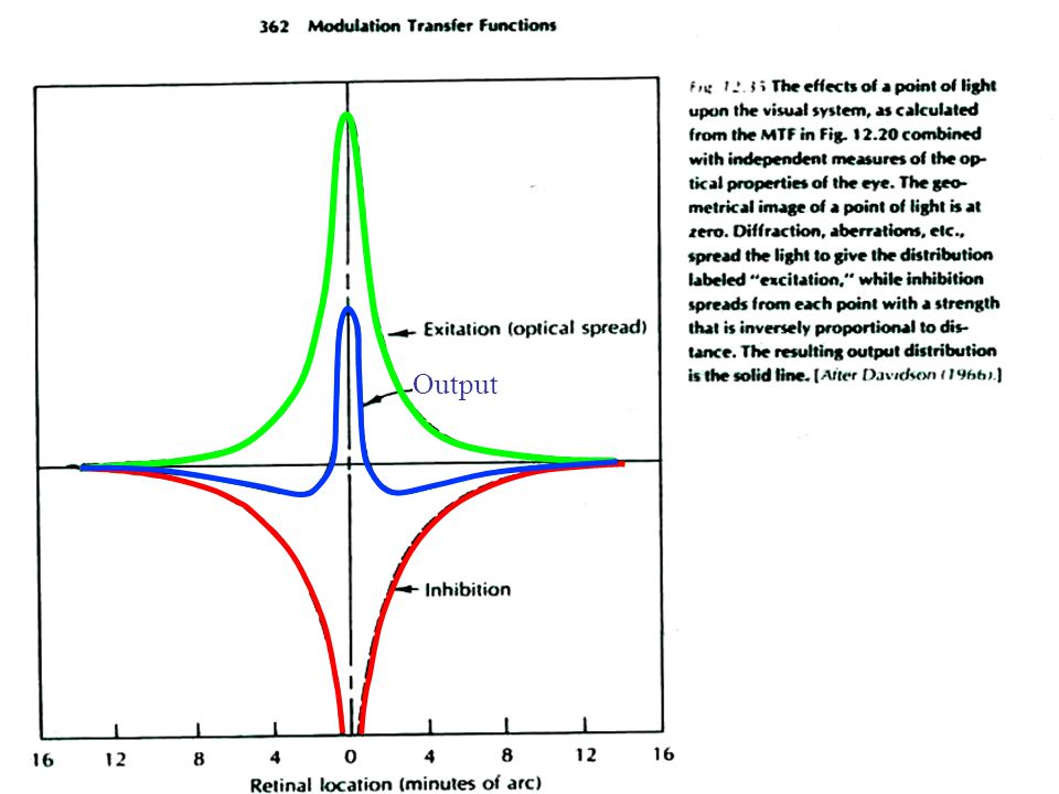
Why does our sensitivity cut off at high frequency? Answ. The PSF. Optical degradation limits spatial resolution.

90
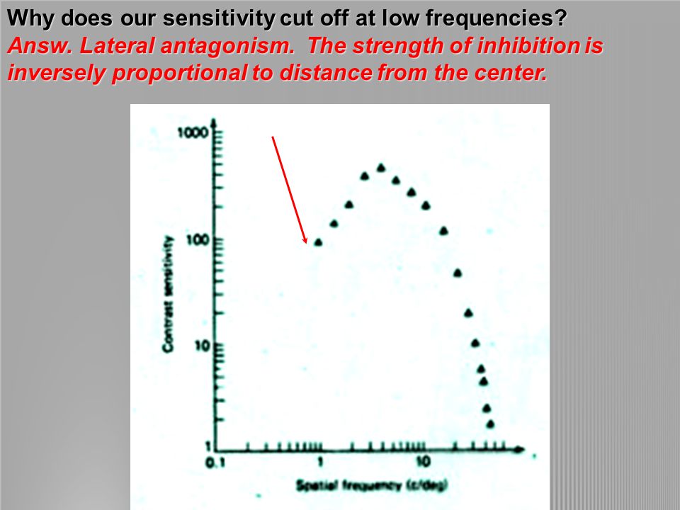
Why does our sensitivity cut off at low frequencies? Answ. Lateral antagonism. The strength of inhibition is inversely proportional to distance from the center.

92
Output

93
Finally, multiple parallel processing streams in our spatial system. Each stream is made up of different frequency-tuned cells (i.e., the size of RF). Evidence for this comes from adaptation and masking studies..
. Evidence for this comes from adaptation and masking studies...")
94
Size of RF can encode the scale of image

95
Explaining the spatial contrast sensitivity function [ The shape of the spatial contrast sensitivity function reflects the properties of the receptive fields that mediate our perception of spatial detail. Neurons with small receptive fields respond to high spatial frequencies. Neurons with large receptive fields respond to low spatial frequencies. The shape of the contrast sensitivity function indicates that there are fewer, less responsive receptive fields at extreme sizes.

96
Low adapt high adapt

97
bottom top c/deg S S Test appears “lower” in frequency Test appears “higher” in frequency test

98
Sensitivity shift towards 3 After prolonged adaptation to a Adapt to a spatial frequency est

101
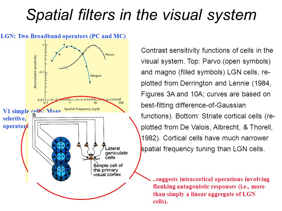
Spatial filters in the visual system C Contrast sensitivity functions of cells in the visual system. Top: Parvo (open symbols) and magno (filled symbols) LGN cells, re- plotted from Derrington and Lennie (1984, Figures 3A and 10A; curves are based on best-fitting difference-of-Gaussian functions). Bottom: Striate cortical cells (re- plotted from De Valois, Albrecht, & Thorell, 1982). Cortical cells have much narrower spatial frequency tuning than LGN cells. LGN: Two Broadband operators (PC and MC) V1 simple cells: More selective, narrowband operators..suggests intracortical operations involving flanking antagonistic responses (i.e., more than simply a linear aggregate of LGN cells).
 and magno (filled symbols) LGN cells, re- plotted from Derrington and Lennie (1984, Figures 3A and 10A; curves are based on best-fitting difference-of-Gaussian functions). Bottom: Striate cortical cells (re- plotted from De Valois, Albrecht, & Thorell, 1982). Cortical cells have much narrower spatial frequency tuning than LGN cells. LGN: Two Broadband operators (PC and MC) V1 simple cells: More selective, narrowband operators..suggests intracortical operations involving flanking antagonistic responses (i.e., more than simply a linear aggregate of LGN cells)..")
102
NOTE: Behavioral evidence from adaptation and masking studies (superimposing gratings of slightly different spatial frequencies and measuring resultant changes in sensitivity) correlates well with cortical cell measurements!
 correlates well with cortical cell measurements!")
103
Spatiotemporal contrast sensitivity We can examine spatial and temporal sensitivity together by measuring the visibility of flickering gratings. Spatial and temporal parameters interact, so there is a trade-off between spatial acuity and temporal acuity. At low temporal frequencies, sensitivity is highest at medium spatial frequencies; at high temporal frequencies, sensitivity is highest at low spatial frequencies. Spatiotemporal contrast sensitivity probably reflects the contribution of two parallel pathways or channels of processing. At low temporal frequencies contrast sensitivity reflects activity of cells in the parvo division; at high temporal frequencies contrast sensitivity reflects activity of cells in the magno division.

104
Steady sinusoidal gratings Low spatial frequency (cpd) gratings with varying temporal frequencies (c/sec or Hz). Lesioned parvocelluar stream (low pass) Lesioned parvocelluar stream (band pass) Lesioned magnocelluar stream (low pass) Lesioned magnocelluar stream (band pass)
 Lesioned parvocelluar stream (band pass) Lesioned magnocelluar stream (low pass) Lesioned magnocelluar stream (band pass).")
105
[ Top: Space–time plot of a spatial grating that repetitively reverses in contrast over time. The grating’s spatial frequency is defined by the rate of contrast alternation across space (horizontal slices through the panel). The grating’s flicker temporal frequency is defined by the rate of contrast alternation across time (vertical slices through the panel). B Bottom: Contrast sensitivity for flickering gratings as a function of their spatial frequency (horizontal axis) and temporal frequency (different curves), re-drawn from Robson (1966). Spatial sensitivity is band-pass at low temporal frequencies (filled squares), but low-pass at high temporal frequencies (filled circles). Spatiotemporal contrast sensitivity
. The grating’s flicker temporal frequency is defined by the rate of contrast alternation across time (vertical slices through the panel). B Bottom: Contrast sensitivity for flickering gratings as a function of their spatial frequency (horizontal axis) and temporal frequency (different curves), re-drawn from Robson (1966). Spatial sensitivity is band-pass at low temporal frequencies (filled squares), but low-pass at high temporal frequencies (filled circles). Spatiotemporal contrast sensitivity.")
106
Functional significance of multiple spatial filters The visual system uses spatial filters in several important tasks: Edge localization Texture analysis Stereo and motion analysis

107
Edge localization 1: Vernier acuity [ We can assign locations to (localise) luminance edges with very high precision. Vernier acuity is typically 1/6 th of the distance between adjacent photoreceptors.

108
Edge localization 2: Explaining Vernier acuity [ The retinal image of an edge is spread optically over a distance covered by 5 or 6 receptors (top graph). A very small (fine-scale) change in edge position causes the response of each receptor to change by up to 25% (middle and bottom graphs). A small center–surround receptive field computing the difference between adjacent receptor responses would detect the shift in position. Large receptive fields detect larger shifts in position. A number of computational theories have been proposed for how information about edge position is extracted from receptive field responses. (i.e., fovea)
 change in edge position causes the response of each receptor to change by up to 25% (middle and bottom graphs). A small center–surround receptive field computing the difference between adjacent receptor responses would detect the shift in position. Large receptive fields detect larger shifts in position. A number of computational theories have been proposed for how information about edge position is extracted from receptive field responses. (i.e., fovea).")
109
David Marr (1980) Spatial scale & position (Edge Detection) The Raw Primal Sketch derived from a computational approach to images. dy/dx -- slope of function y [or f(x)]; d 2 y/dx 2 -- zero crossings of f(x).
]; d 2 y/dx 2 -- zero crossings of f(x)..")
Similar presentations


 Presented by: CHEN Wei (Rosary) Supervisor: Dr. Richard So.>")


 Related color: color.>")
 Related color: color.>")
 Related color: color perceived to belong to.>")
![MSU CSE 803 Stockman Fall 2009 Vectors [and more on masks] Vector space theory applies directly to several image processing/representation problems.](/16/5019143/big_thumb.jpg "MSU CSE 803 Stockman Fall 2009 Vectors [and more on masks] Vector space theory applies directly to several image processing/representation problems.>")

![1 MSU CSE 803 Fall 2014 Vectors [and more on masks] Vector space theory applies directly to several image processing/representation problems.](/17/5291738/big_thumb.jpg "1 MSU CSE 803 Fall 2014 Vectors [and more on masks] Vector space theory applies directly to several image processing/representation problems.>")

