2. Table 8.1 pg. 202 Review

3. 08_05 DOLLARS QUANTITY MC ATC AVC Fig. 8.9 Review: Generic Cost Curves

4. Review: Profit Maximization 06_08 Total costs 100  200 100 300 400 123450 12345 0 QUANTITY PRODUCED DOLLARS Total revenue Profits DOLLARS Fig 6.8 Profit Max Rule: MR=MC

5. 08_05 DOLLARS QUANTITY MC ATC AVC Fig. 8.9 Zero Economic Profit (P = MC = ATC) P2P2 Break Even Point

6. Fig. 8.9 Negative Economic Profits (AVC<P<ATC) P3P3 Negative Profits Q2Q2

7. 08_05 DOLLARS QUANTITY MC ATC AVC Fig. 8.10 Shutdown Point (P < AVC) P Negative Profits Q Shutdown Point

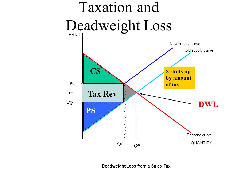
8. Measuring Efficiency Consumer Surplus + Producer Surplus= Total Social Profit Deadweight Loss: The loss in total social profit due to an inefficient level of production. Examples: Taxes and Price Controls

10. Taxation and Deadweight Loss 07_08A Old supply curve Demand curve QUANTITY PRICE Deadweight Loss from a Sales Tax New supply curve S shifts up by amount of tax P* Tax Rev DWL CS PS Pp Pc Qt Q*

11. Quantity MC = S ATC Price or Cost ($) q0q0 S0S0 D0D0 Q0Q0 Price ($) Quantity P0P0 P0P0 Typical FirmIndustry or Market Short Run Equilbrium Firm: P 0 = MR = MC Industry: Q d = Q s @ P 0 Long Run Equilbrium Firm: Econ  = 0 Industry: Firms @ Min LRATC Long Run Equilibrium Condtions

12. (1)Many small firms Homogenous product. (2)Identical product (3)Perfect Information. Total Knowledge (4) Free entry and exit. Results Price taker with no market power. Firm believes it can sell it all if it takes market price. Always P=MR=MC @ min ATC Perfectly Competitive Market Assumptions

13. Quantity MC = S ATC Price or Cost ($) q0q0 S0S0 D0D0 Q0Q0 Price ($) Quantity Typical FirmIndustry or Market D1D1 Q1Q1 P1P1 P1P1 q1q1 S1S1 Long Run Competitive Equilibrium Model Demand Shock: Shift Demand Left Loss Q2Q2 q2q2 P0P0 P 2 = P0P0

14. Quantity MC = S ATC Price or Cost ($) q0q0 S0S0 D0D0 Q0Q0 Price ($) Quantity Typical FirmIndustry or Market D1D1 Q1Q1 P1P1 P1P1 q1q1 S1S1 Q2Q2 q2q2 P0P0 P0P0 P 2 = Long Run Competitive Equilibrium Model Demand Shock: Shift Demand Right Profits

15. Lesson 15 Monopoly: Part 1

16. What is a Monopoly? Many small firms Homogeneous Good Perfect Information No Barriers to Entry or Ex it Small Output Compared to Industry Price taker No market power Is effiecient 1 firm Unique product Perfect knowledge that firm has you Barriers to Entry or Exit--Blocked Price Setter Extreme market power Is inefficient Competitive Firm Monopoly

17. Quantity Price ($) Quantity D0D0 Price ($) Competitive Firm’s ViewMonopoly’s View D0D0 For Perfectly Competitive Markets: Demand Curve: Flat / Horizontal No Market Power / Price Taker For a Monopoly: Demand Curve: Negatively Sloped Market Power / Price “Maker” Model of a Monopoly Market Power

18. What is the Profit Maximizing Rule 10_05 Total costs Total revenue Maximum QUANTITY DOLLARS Slope equals price. Slope equals marginal cost. QUANTITY DOLLARS Competitive Firm Monopoly Slope equals marginal revenue. Slope equals marginal cost. MR=MC

19. 10_04 19283745610 200 150 100 50 0 DOLLARS QUANTITY Marginal cost ( MC ) Demand Marginal revenue ( MR ) Profit Max is Where MR = MC (fig 10.4)

20. TR = P * Q  = TR - TC TC = ATC * Q Quantity MC ATC Price or Cost ($) Monopoly D MR QMQM PMPM Model of a Monopoly Positive Economic Profits

21. TC = ATC * Q TR = P * Q Quantity MC ATC Price or Cost ($) Monopoly QMQM PMPM  = TR - TC D MR Model of a Monopoly Negative Economic Profits

22. Model of a Monopoly Board Problem Market:Cadet Comforters Scenario:Q D = 40 - PwhereQ: comforters / week TC = Q 2 + 4Q + 58P: $ / comforter Question:(a)Calulate the MR and MC functions. (b)Depict the following curves on a graph: D, MR, MC. (c)Determine the equilibrium price and quantity if the firm acts like a perfectly competitive firm. Depict P PC and Q PC on the graph. Calculate the firm’s profits. (d)Determine the equilibrium price and quantity if the firm acts like a monopoly. Depict P M and Q M on the graph. Calculate the firm’s profits.

23. Model of a Monopoly Board Problem Solution (a) P=40 - Q TR=P*QMC=dATC / dQ MR=40 - 2Q=(40 - Q)QMC=2Q + 4 TR=40Q - Q 2 MR=dTR / dQ MR=40 - 2Q (b)See graph. (c)Set P = MC: 40 - Q=2Q + 4 P = 40 - Q 3Q =36=40 - 12 Q=12 comforters / week P=$28 / comforter  =TR - TC = (P*Q) - (Q 2 + 4 Q + 58) =336 - 250  =$86 / week (d)Set MR = MC: 40 - 2Q=2Q + 4 P = 40 - Q 4Q =36=40 - 9 Q=9 comforters / week P=$31 / comforter  =TR - TC = (P*Q) - (Q 2 + 4 Q + 58) =279 - 175  =$104 / week

24. Model of a Monopoly Board Problem Solution Quantity Price or Cost ($) Cadet Comforter Firm D = PMR MC P PC = 28 P M = 31 20400 0 20 40 QMQM 9 Q PC 12

25. Creating Money--Deposit Expansion DepositsLoansReserves BankTwo10.009.001.00 BankThree9.008.10.90 BankFour8.107.29.81 Etc. Final Sum100.009010 The Simple Multiplier: BR=r * D, solve for D BR/r=D or D=BR * 1/r The Simple Multiplier is 1/r Deposits Expand to D*1/r

26. Deriving The Money Multiplier MB=CU+BR which the Fed controls We know that M=CU + D Substitute in CU=kD and we get M=kD+D or M= (k+1)D We also know that BR=r*D and that MB=CU+BR Substitute in and MB=kD+rD or MB=(k+r)D To find the link divide M by MB: (k+1)D/(k+r)D The Money Multiplier = (k+1)/(k+r) The multiple by which the money supply changes due to a change in the monetary base.

27. Lesson 27: Investment in New Capital

28. What is the impact on I if C increases? Fig. 22.9 22_09 R 2.5 5.0 7.5 0.0 65.062.567.5 C Y (a) Consumption Share R 2.5 5.0 7.5 0.0 15.012.517.5 I Y (b) Investment Share R 2.5 5.0 7.5 0.0 807585 R 2.5 5.0 7.5 0.0 2.5 X Y (c) Net Exports Share -2.5 PERCENT NG Y (d) Nongovernment Share Investment decreases as interest rates rise.

29. “We figure it was HERE when the recession officially began.” Taylor p. 677 Lesson 31 Aggregate Expenditure

30. The Rounds of the Multiplier Process fig 26.2 26_02 BILLIONS OF DOLLARS 1111029368547 300 250 200 150 100 50 0 $250 billion ROUND MPC =.6

31. Graphically –Determine the shift in the AE Line –Determine the shift in Real GDP –Divide Real GDP Shift by AE Line Shift to get Multiplier Algebraically –Derivation on page 703 –Multiplier = 1 / (1-MPC) Example: If MPC =.8, Multiplier = 5 How to Calculate the Multiplier

32. 45  line Boom AE line e c d Normal AE line Recession AE line INCOME OR REAL GDP (TRILLIONS OF 1992 DOLLARS) 5.756.506.256.00 6.50 SPENDING (TRILLIONS OF 1992 DOLLARS) 6.25 6.00 5.75 25_11B SPENDING (TRILLIONS OF 1992 DOLLARS d 6.25 6.50 6.00 5.75 Year 1Year 3Year 2 c e b a (Boom) (Real GDP= potential GDP) (Recession) Spending Balance Recessions and Booms fig. 25.11