1. Chapter 4 – Bipolar Junction Transistors (BJTs)
Introduction

2. Physical Structure and Modes of Operation
A simplified structure of the npn transistor.

3. Physical Structure and Modes of Operation
A simplified structure of the pnp transistor.

4. Physical Structure and Modes of Operation
Mode EBJ CBJ
Active Forward Reverse
Cutoff Reverse Reverse
Saturation Forward Forward

5. Operation of The npn Transistor Active Mode
Current flow in an npn transistor biased to operate in the active mode, (Reverse current components due to drift of thermally generated minority carriers are not shown.)

6. Operation of The npn Transistor Active Mode
Profiles of minority-carrier concentrations in the base and in the emitter of an npn transistor operating in the active mode; vBE  0 and vCB  0.

7. Operation of The npn Transistor Active Mode
The Collector Current
The Base Current
Physical Structure and Modes of Operation

8. Equivalent Circuit Models
Large-signal equivalent-circuit models of the npn BJT operating in the active mode.

9. The Constant n
The Collector-Base Reverse Current
The Structure of Actual Transistors

10. The pnp Transistor
Current flow in an pnp transistor biased to operate in the active mode.

11. The pnp Transistor
Two large-signal models for the pnp transistor operating in the active mode.

12. Circuit Symbols and Conventions

13. Circuit Symbols and Conventions

14. Example 4.1 C B E

15. Example 4.1

16. Example 4.1

18. Exercise 4.8

19. Exercise 4.9

20. The Graphical Representation of the Transistor Characteristics

21. The Graphical Representation of the Transistor Characteristics
Temperature Effect (10 to 120 C)

22. Dependence of ic on the Collector Voltage
The iC-vCB characteristics for an npn transistor in the active mode.

23. Dependence of ic on the Collector Voltage

24. Dependence of ic on the Collector Voltage – Early Effect
VA – 50 to 100V
(a) Conceptual circuit for measuring the iC-vCE characteristics of the BJT. (b) The iC-vCE characteristics of a practical BJT.

25. Dependence of ic on the Collector Voltage – Early Effect

26. Nested DC Sweeps

27. Example

28. Example

29. Example

30. Monte Carlo Analysis – Using PSpice

31. Monte Carlo Analysis – Using PSpice

32. Monte Carlo Analysis – Using PSpice

33. Monte Carlo Analysis – Using PSpice
Probe Output
Ic(Q), Ib(Q), Vce

34. The Transistor As An Amplifier
(a) Conceptual circuit to illustrate the operation of the transistor of an amplifier.
(b) The circuit of (a) with the signal source vbe eliminated for dc (bias) analysis.
The Collector Current and The Transconductance
The Base Current and the Input Resistance at the Base
The Emitter Current and the Input Resistance at the Emitter

35. The Transistor As An Amplifier
Linear operation of the transistor under the small-signal condition: A small signal vbe with a triangular waveform is superimpose din the dc voltage VBE. It gives rise to a collector signal current ic, also of triangular waveform, superimposed on the dc current IC. Ic = gm vbe, where gm is the slope of the ic - vBE curve at the bias point Q.

36. Small-Signal Equivalent Circuit Models
Two slightly different versions of the simplified hybrid- model for the small-signal operation of the BJT. The equivalent circuit in (a) represents the BJT as a voltage-controlled current source ( a transconductance amplifier) and that in (b) represents the BJT as a current-controlled current source (a current amplifier). 

37. Small-Signal Equivalent Circuit Models
Two slightly different versions of what is known as the T model of the BJT. The circuit in (a) is a voltage-controlled current source representation and that in (b) is a current-controlled current source representation. These models explicitly show the emitter resistance re rather than the base resistance r featured in the hybrid- model.

38. Signal waveforms in the circuit of Fig. 4.28.

39. Fig Example 4.11: (a) circuit; (b) dc analysis; (c) small-signal model; (d) small-signal analysis performed directly on the circuit.

40. Fig. 4.34 Circuit whose operation is to be analyzed graphically.

41. Fig Graphical construction for the determination of the dc base current in the circuit of Fig

42. Fig Graphical construction for determining the dc collector current IC and the collector-to-emmiter voltage VCE in the circuit of Fig

43. Fig Graphical determination of the signal components vbe, ib, ic, and vce when a signal component vi is superimposed on the dc voltage VBB (see Fig. 4.34).

44. Fig Effect of bias-point location on allowable signal swing: Load-line A results in bias point QA with a corresponding VCE which is too close to VCC and thus limits the positive swing of vCE. At the other extreme, load-line B results in an operating point too close to the saturation region, thus limiting the negative swing of vCE.

45. Fig The common-emitter amplifier with a resistance Re in the emitter. (a) Circuit. (b) Equivalent circuit with the BJT replaced with its T model (c) The circuit in (b) with ro eliminated.

46. Fig. 4. 45 The common-base amplifier. (a) Circuit
Fig The common-base amplifier. (a) Circuit. (b) Equivalent circuit obtained by replacing the BJT with its T model.

47. Fig. 4. 46 The common-collector or emitter-follower amplifier
Fig The common-collector or emitter-follower amplifier. (a) Circuit. (b) Equivalent circuit obtained by replacing the BJT with its T model. (c) The circuit in (b) redrawn to show that ro is in parallel with RL. (d) Circuit for determining Ro.

48. A General Large-Signal Model For The BJT: The Ebers-Moll Model
ISC > ISE (2-50)
An npn resistor and its Ebers-Moll (EM) model. ISC and ISE are the scale or saturation currents of diodes DE (EBJ) and DC (CBJ).
More General – Describe Transistor in any mode of operation.
Base for the Spice model.
Low frequency only

49. A General Large-Signal Model For The BJT:
The Ebers-Moll Model

50. A General Large-Signal Model For The BJT:
The Ebers-Moll Model – Terminal Currents

51. A General Large-Signal Model For The BJT:
The Ebers-Moll Model – Forward Active Mode
Since vBC is negative and its magnitude
Is usually much greater than VT the
Previous equations can be approximated as

52. A General Large-Signal Model For The BJT:
The Ebers-Moll Model – Normal Saturation

53. A General Large-Signal Model For The BJT:
The Ebers-Moll Model – Reverse Mode
Note that the currents indicated have positive values. Thus, since ic = -I2 and iE = -I1, both iC and IE will be negative. Since the roles of the emitter and collector are interchanged, the transistor in the circuit will operate in the active mode (called the reverse active mode) when the emitter-base junction is reverse-biased. In such a case
I1 = beta_R . IB
This circuit will saturate (reverse saturation mode) when the emitter-base junction becomes forward-biased.
I1/IB < beta_R I1 IB I2

54. A General Large-Signal Model For The BJT:
The Ebers-Moll Model – Reverse Saturation
We can use the EM equations to find the expression of VECSat
From this expression, it can be seen that the minimum VECSat is obtained when I1 = This minimum is very close to zero.
The disadvantage of the reverse saturation mode is a relatively long turnoff time.

55. A General Large-Signal Model For The BJT:
The Ebers-Moll Model – Example

56. A General Large-Signal Model For The BJT:
The Ebers-Moll Model – Example

57. A General Large-Signal Model For The BJT:
The Ebers-Moll Model – Transport Model npn BJT
The transport model of the npn BJT. This model is exactly equivalent to the Ebers-Moll model. Note that the saturation currents of the diodes are given in parentheses and iT is defined by Eq. (4.117).

58. Basic BJT Digital Logic Inverter.
vi high (close to power supply) - vo low
vi low vo high
Basic BJT digital logic inverter.

59. Basic BJT Digital Logic Inverter.
Sketch of the voltage transfer characteristic of the inverter circuit of Fig for the case RB = 10 k, RC = 1 k,  = 50, and VCC = 5V. For the calculation of the coordinates of X and Y refer to the text.

60. The Voltage Transfer Characteristics
(a) The minority-carrier concentration in the base of a saturated transistor is represented by line (c). (b) The minority-carrier charge stored in the base can de divided into two components: That in blue produces the gradient that gives rise to the diffusion current across the base, and that in gray results in driving the transistor deeper into saturation.

61. Complete Static Characteristics, Internal Impedances,
and Second-Order Effects – Common Base
Avalanche
Saturation
Slope
The ic-vcb or common-base characteristics of an npn transistor. Note that in the active region there is a slight dependence of iC on the value of vCB. The result is a finite output resistance that decreases as the current level in the device is increased.

62. Complete Static Characteristics, Internal Impedances,
and Second-Order Effects – Common Base
The hybrid- model, including the resistance r, which models the effect of vc on ib.

63. Complete Static Characteristics, Internal Impedances,
and Second-Order Effects – Common-Emitter
Common-emitter characteristics. Note that the horizontal scale is expanded around the origin to show the saturation region in some detail.

64. Complete Static Characteristics, Internal Impedances,
and Second-Order Effects – Common-Emitter
An expanded view of the common-emitter characteristics in the saturation region.

65. The Transistor Beta

66. Transistor Breakdown

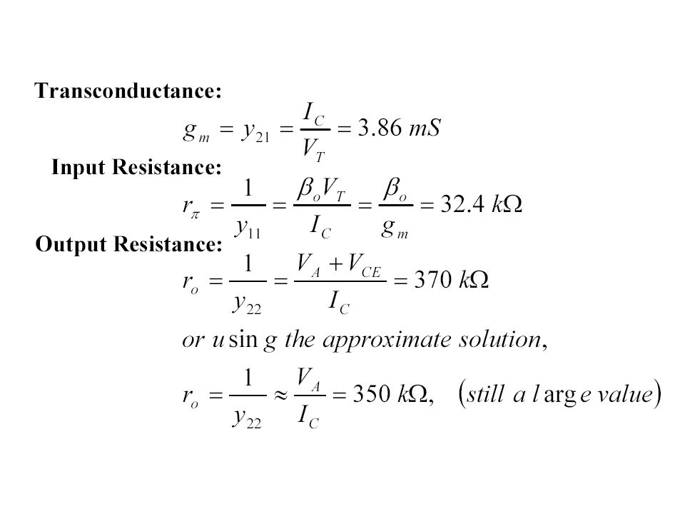
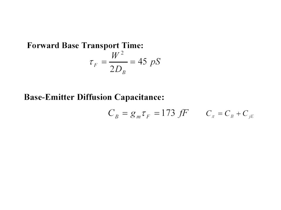
67. Internal Capacitances of a BJT

68. The Cut-Off Frequency

69. The Spice BJT Model and Simulation Examples

70. The Spice BJT Model and Simulation Examples

71. The Spice BJT Model and Simulation Examples

72. The Spice BJT Model and Simulation Examples
.model Q2N2222-X NPN(
Is=14.34f
Xti=3
Eg=1.11
Vaf=74.03
Bf=200
Ne=1.307
Ise=14.34f
Ikf=.2847
Xtb=1.5
Br=6.092
Nc=2
Isc=0
Ikr=0
Rc=1
Cjc=7.306p
Mjc=.3416
Vjc=.75
Fc=.5
Cje=22.01p
Mje=.377
Vje=.75
Tr=46.91n
Tf=411.1p
Itf=.6
Vtf=1.7
Xtf=3
Rb=10)
*National pid=19
case=TO bam creation

73. The Spice BJT Model and Simulation Examples

74. BJT Modeling - Idealized Cross Section of NPN BJT
BJT Modeling - Idealized Cross Section of NPN BJT

77. The Spice BJT Model and Simulation Examples