Download presentation
Presentation is loading. Please wait.

1
Measuring CO 2 from Space Approach: Collect spectra of CO 2 and O 2 and absorption in sunlight reflected from the surface and scattered from the atmosphere Normalize CO 2 absorption with O 2 absorption to remove effects of varying surface pressure & topography and minimize aerosol/cloud effects Measurements yields total CO 2 column with high sensitivity to CO 2 near surface Sensitivity to CO 2

2
The NASA Orbiting Carbon Observatory (OCO) Approach: Collect spectra of CO 2 and O 2 absorption in reflected sunlight Use these data to resolve variations in the column averaged CO 2 dry air mole fraction, X CO2 over the sunlit hemisphere Validate measurements to ensure X CO2 accuracies of 1 - 2 ppm (0.3 - 0.5%) on regional scales at monthly intervals OCO will acquire the space-based data needed to identify CO 2 sources and sinks on regional scales over the globe and quantify their variability over the seasonal cycle
 Approach: Collect spectra of CO 2 and O 2 absorption in reflected sunlight Use these data to resolve variations in the column averaged CO 2 dry air mole fraction, X CO2 over the sunlit hemisphere Validate measurements to ensure X CO2 accuracies of ppm ( %) on regional scales at monthly intervals OCO will acquire the space-based data needed to identify CO 2 sources and sinks on regional scales over the globe and quantify their variability over the seasonal cycle")
3
Making Precise CO 2 Measurements from Space Scattering from Clouds/Aerosols, H 2 O, Temperature O 2 A-band CO 2 1.61 m CO 2 2.06 m High resolution spectra of reflected sunlight in near-IR CO 2 and O 2 bands used to retrieve X CO2 –1.61 m CO 2 band: Column CO 2 –2.06 m CO 2 band: Column CO 2, clouds/aerosols –0.76 m O 2 A-band: Surface pressure, clouds/aerosols Self-consistent retrieval, no additional information needed High spectral resolution enhances sensitivity and minimizes biases Scattering from Clouds/Aerosols, Surface Pressure, Temperature Column CO 2 Sensitivity to CO 2

4
On-orbit Measurement Strategy Optimized to minimize bias and yield high Signal/Noise observations over the globe Nadir Observations: tracks local nadir + Small footprint (< 3 km 2 ) isolates cloud-free scenes and reduces biases from spatial inhomogeneities over land Low Signal/Noise over dark ocean Glint Observations: views “glint” spot + Improves Signal/Noise over oceans More interference from clouds Nadir Local Nadir Glint Spot Ground Track Glint
 isolates cloud-free scenes and reduces biases from spatial inhomogeneities over land Low Signal/Noise over dark ocean Glint Observations: views glint spot + Improves Signal/Noise over oceans More interference from clouds Nadir Local Nadir Glint Spot Ground Track Glint")
5
4 5 OCO Will Provide Dramatically Improved Spatial and Temporal CO 2 Sounding ~200 samples per degree of latitude as OCO moves along its orbit track on day side of the Earth Uniform sampling of land and ocean 7 M soundings per 16-day repeat cycle

6
Effects of Clouds and Aerosols Chevallier et al. 2006 OCO 3-Days OCO 1-Day GLAS Satellite: Clouds reduce number of usable samples, but OCO still collects thousands of samples on regional scales each month. Clear-sky frequency vs. spatial resolution computed using the MODIS 1 km cloud product Bösch et al., JGR, 2006 Red points show cloud-free hits along each orbit track

7
January July Global Single Sounding X CO2 Retrieval Error Surface climatology + AOD histogram (CCM3 model over ice) No systematic errors included here (i.e. perfect Forward Model) X CO2 Error (ppm) Single Sounding X CO2 Error (ppm) Nadir Glint Glint effect for snow not taken into account
 X CO2 Error (ppm) Single Sounding X CO2 Error (ppm) Nadir Glint Glint effect for snow not taken into account.")
8
January July Number of Cloud-free OCO Soundings MODIS 1 km 2 cloud mask accumulated to effective OCO pixel size Nadir (SZA < 85 o ) Glint (SZA < 75 o ) Number of Soundings per 16 day Repeatcycle and 1 0 x1 0 Bin
 Glint (SZA < 75 o ) Number of Soundings per 16 day Repeatcycle and 1 0 x1 0 Bin")
9
Ensemble X CO2 Retrieval Error per Repeatcycle Surface climatology + AOD climatology (for AOD < 0.3) + number of cloud-free soundings (Remark: only subset of cloud-free soundings might be retrieved) Again: No systematic errors included here (i.e. perfect Forward Model) January July Nadir (SZA < 85 o ) Glint (SZA < 75 o ) Ensemble X CO2 Error per 16 day Repeatcycle and 1 0 x1 0 Bin (ppm) Glint (SZA < 75 o )
 January July Nadir (SZA < 85 o ) Glint (SZA < 75 o ) Ensemble X CO2 Error per 16 day Repeatcycle and 1 0 x1 0 Bin (ppm) Glint (SZA < 75 o ).")
10
OCO Summary OCO has the potential to provide accurate retrieval of CO 2 columns that will enable computation of CO 2 fluxes over regional scales on seasonal time scales OCO has a narrow swath width of 10 km and will not provide global coverage Japanese CO2 instrument (GOSAT) will be launched at same time as OCO and combining both datasets can largely increase sampling
 will be launched at same time as OCO and combining both datasets can largely increase sampling")
11
OCOSCIAMACHY/ENVISAT LaunchScheduled for 12/2008March 2002 ObjectiveCO 2 solelyMany atmospheric trace gases ModesNadir, glint, targetNadir (limb, occultation) Range3 narrow NIR bands8 Channels from UV to NIR ResolutionHigh: 0.05 nm – 0.1 nmLow/medium: 0.2 – 1.5 nm Ground Pixel3 km 2 60 x 30 km 2 RetrievalOptimal EstimationFSI-WFM (linear least-square fit) ENVISAT/SCIAMACHY OCO Comparison of SCIAMACHY and OCO
 Range3 narrow NIR bands8 Channels from UV to NIR ResolutionHigh: 0.05 nm – 0.1 nmLow/medium: 0.2 – 1.5 nm Ground Pixel3 km 2 60 x 30 km 2 RetrievalOptimal EstimationFSI-WFM (linear least-square fit) ENVISAT/SCIAMACHY OCO Comparison of SCIAMACHY and OCO")
12
Carbon Fusion Oct07 CO 2 Time Series for N-America from SCIAMACHY

13
CO 2 Time Series for Siberia from SCIAMACHY

14
Comparison of SCIAMACHY to Aircraft Observations at Surgut Better agreement at 1.5-2.0 km

15
Comparison of SCIAMACHY to Surface CO 2 : USA (±5°lon/lat of site) SCIAMACHY = Red Surface = Blue Difference to Mean ValueDirect Comparison
 SCIAMACHY = Red Surface = Blue Difference to Mean ValueDirect Comparison")
18
SCIAMACHY Summary Encouraging first results from the FSI algorithm Good agreement with FT stations at Egbert & Park Falls (bias -2 to -4%) Good agreement with TM3 model (more uptake in summer) Good agreement with aircraft data over Siberia Good agreement with AIRS CO 2 (accounting for different vertical sensitivity) Good agreement with surface network Good correlation with vegetation spatial distribution Key point: SCIAMACHY can track changes in near surface CO 2 (although SCIAMACHY is a non-ideal instrument for CO 2 ) Comparison of vegetation indices vs. CO 2 indicate SCIAMACHY can track biological signal at regional level (though at limit of sensitivity)
.")
19
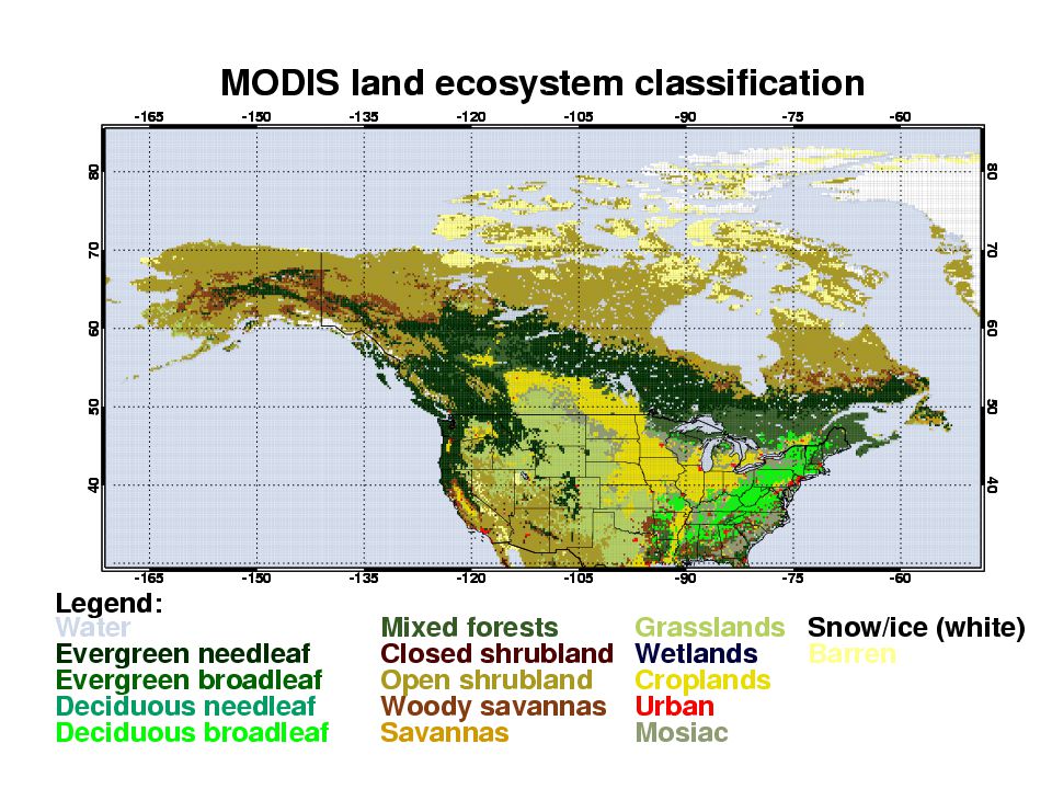
1.To integrate the ECOSSE soil model together with the JULES (Joint UK Land Environment Simulator) vegetation model into the Lagrangian transport model NAME 2.To model CO 2 fields for the UK/Scotland region for several weeks during summer/autumn for the years 2006 and 2007 with and without fluxes from the ECOSSE model 3.To generate atmospheric CO 2 for UK/Scotland region the from SCIAMACHY/ENVISAT for the same time period including detailed assessment of the uncertainties 4.To assess the capabilities of SCIAMACHY for observing carbon fluxes released from the soil 5.To simulate CO 2 fields for the UK/Scotland region using future land-use change scenarios 6.To assess the capabilities of future satellite instruments (OCO, GOSAT) to observe and monitor carbon fluxes due to land-use change Preparatory work on the use of remote-sensing techniques for the detecting and monitoring of GHG emissions from the Scottish land use sector People: Gennaro Cappelutti, Hartmut Boesch, Paul Monks, Alan Hewitt, Joerg Kaduk
 vegetation model into the Lagrangian transport model NAME 2.To model CO 2 fields for the UK/Scotland region for several weeks during summer/autumn for the years 2006 and 2007 with and without fluxes from the ECOSSE model 3.To generate atmospheric CO 2 for UK/Scotland region the from SCIAMACHY/ENVISAT for the same time period including detailed assessment of the uncertainties 4.To assess the capabilities of SCIAMACHY for observing carbon fluxes released from the soil 5.To simulate CO 2 fields for the UK/Scotland region using future land-use change scenarios 6.To assess the capabilities of future satellite instruments (OCO, GOSAT) to observe and monitor carbon fluxes due to land-use change Preparatory work on the use of remote-sensing techniques for the detecting and monitoring of GHG emissions from the Scottish land use sector People: Gennaro Cappelutti, Hartmut Boesch, Paul Monks, Alan Hewitt, Joerg Kaduk")
20
SCIAMACHY Monthly Mean CO 2 for UK

21
SCIAMACHY CO 2 for Overpass over UK SCIAMACHY orbit geometry and clouds largely reduce number of available soundings per overpass: – SCIAMACHY has global coverage every 3-4 days – Large ground pixel size (30x60 km 2 ) of SCIAMACHY result in frequent cloud perturbations OCO-type retrieval could increase the number of useful soundings (normalization with O 2 column) and decrease the sensitivity to small cloud perturbations
 of SCIAMACHY result in frequent cloud perturbations OCO-type retrieval could increase the number of useful soundings (normalization with O 2 column) and decrease the sensitivity to small cloud perturbations")
22
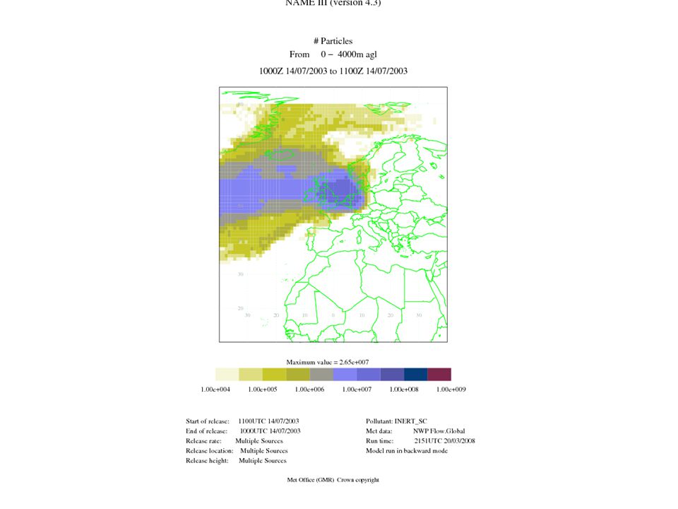
UK Met Office NAME NAME is the UK met office dispersion model: A number of particles are released from a start point. The individual particles are followed and are at a new location at each time step, based on the wind fields. Particles are followed for a set time period or until they leave a target region. Model output might include surface contact time. Model can be run with time forward or backwards. Name can be coupled with inversion scheme for surface fluxes

26
Setup of NAME Model Setup of Name: Run backwards from Scotland/UK and store the surface contact time per grid box Temporal and spatial resolution: - currently 1x1 grid for several altitudes and 15 min. timesteps - finer resolution possible over source region, currently 15 min..) Computational requirements: 0.5 hours per day for UK on a 1x1 grid Data requirements: met fields from UKMET Calculation of 3D CO 2 fields: Requires fluxes for each grid box (e.g. as ASCII table)
 Computational requirements: 0.5 hours per day for UK on a 1x1 grid Data requirements: met fields from UKMET Calculation of 3D CO 2 fields: Requires fluxes for each grid box (e.g. as ASCII table).")
27
Questions/Issues Which spatial and temporal resolution is needed. What are the timescales to look at How to interface ECOSSE model with JULES model (for plant photosynthesis and plant respiration) in a consistent way (e.g. litter) Which current and future scenarios are planned? Availability of data ? Should we include other remote sensing information (e.g. CH4) Initialisation of NAME model with CO2 at starting point Inclusion of anthropogenic emissions Summary Project just started (Gennaro will be main person to work on the project) SCIAMACHY CO2 is ‘operationally ‘ retrieved at Leicester with FSI-WFM algorithm Due to clouds and sampling, only few SCIAMACHY soundings will be available on daily basis. Situation will improve with the launch of OCO and GOSAT. Additionally, in-situ surface observations could be used. NAME and JULES model (+expertise) are available at Leicester
 in a consistent way (e.g. litter) Which current and future scenarios are planned. Availability of data . Should we include other remote sensing information (e.g. CH4) Initialisation of NAME model with CO2 at starting point Inclusion of anthropogenic emissions Summary Project just started (Gennaro will be main person to work on the project) SCIAMACHY CO2 is ‘operationally ‘ retrieved at Leicester with FSI-WFM algorithm Due to clouds and sampling, only few SCIAMACHY soundings will be available on daily basis. Situation will improve with the launch of OCO and GOSAT. Additionally, in-situ surface observations could be used. NAME and JULES model (+expertise) are available at Leicester.")
Similar presentations


 Collaborators Hartmut Bösch (Univ Leicester) Rob Spurr (RT Solutions)>")
, Its Use in Inverse Modeling, and Comparisons to AIRS, SCIAMACHY,>")


, Hartmut Bösch (University of Leicester), Rob Spurr (RT Solutions), Yuk Yung.>")
 The Orbiting Carbon Observatory (OCO) Mission Vijay NatrajGe152 Wednesday, 1 March 2006.>")


