1. Types of classical controllers Proportional control –Needed to make a specific point on RL to be closed-loop system dominant pole Proportional plus derivative control (PD control) –Needed to “bend” R.L. into the desired region Lead control –Similar to PD, but without the high frequency noise problem; max angle contribution limited to < 75 deg Proportional plus Integral Control (PI control) –Needed to “eliminate” a non-zero steady state tracking error Lag control –Needed to reduce a non-zero steady state error, no type increase PID control –When both PD and PI are needed, PID = PD * PI Lead-Lag control –When both lead and lag are needed, lead-lag = lead * lag

2. Proportional control design 1.Draw R.L. for given plant 2.Draw desired region for poles from specs 3.Pick a point on R.L. and in desired region Use ginput to get point and convert to complex # 4.Compute 5.Obtain closed-loop TF 6.Obtain step response and compute specs 7.Decide if modification is needed nump=…; denp= …; sysp=tf(nump, denp); rlocus(sysp); use your program from several weeks ago to do all these syscl = feedback(sysc*sysp,1); Gpd=evalfr(sysp,pd); K=1/Gpd; sysc = K; [x,y]=ginput(1); pd=x+j*y;

3. Design steps: 1.From specs, draw desired region for pole. Pick from region, not on RL 2.Compute 3.Select 4.Select: Gpd=evalfr(sysp,pd) phi=pi - angle(Gpd) z=abs(real(pd))+abs(imag(pd)/tan(phi)); Kd=1/abs(pd+z)/abs(Gpd); Kp=z*Kd; PD controller design [x,y]=ginput(1); pd=x+j*y;

4. Lead Control: 1.Draw R.L. for G 2.From specs draw region for desired c.l. poles 3.Select p d from region 4.Let Pick –z somewhere below p d on –Re axis Let Select Approximation to PD Same usefulness as PD [x,y]=ginput(1); z=abs(x); phi1=angle(pd+z); phi2=phi1-phi; [x,y]=ginput(1); pd=x+j*y; Gpd=evalfr(sysp,pd) phi=pi - angle(Gpd) p=abs(real(pd))+abs(imag(pd)/tan(phi2)); K=abs((pd+p)/(pd+z)/Gpd); sysc=tf(K*[1 z],[1 p]); Hold on; rlocus(sysc*sysp);

5. Alternative Lead Control 1.Draw R.L. for G 2.From specs draw region for desired c.l. poles 3.Select p d from region 4.Let Select phipd=angle(pd); phi1=(phipd+phi)/2; phi2=phi1-phi;

6. Lag controller design It has “destabilizing” effect (lag) Not used for improving M P, t r, … Use it to improve e ss Use it when R.L. of G(s) go through the desired region but e ss is too large. –First select K, as in proportional control –Select z, p so that z/p>1, ess*p/z = ess_des

7. Lag Design steps 1.Draw R.L. for G(s). 2.From specs, draw desired pole region 3.Select p d on R.L. & in region 4.Get 5.With that K, compute error constant (K pa, K va, K aa ) from KG(s) 6.From specs, compute K pd, K vd, K ad Kdes = 1/ess; sysol = sysc*sysp; [nol, dol]=tfdata(sysol,'v'); dn0=dol(dol~=0); Kact=nol(end)/dn0(end); P

8. 7.If K act > K des, done else: pick 8.Re-compute 9.Closed-loop simulation & tuning as necessary z=-real(pd)/…; p=z*Kact/Kdes/(1+…); 0.05 or 0.1 K from 8 should be ~1, so 8 is normally skipped.

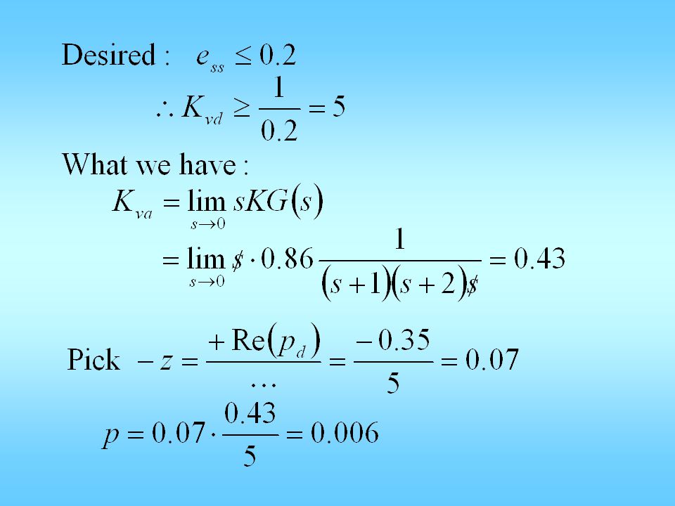
9. Example: Want: Solution: C(s)

10. Draw R.L., and region for desire pole Pick p d on R.L. & in Region pick p d = – 0.35 + j0.5 Since there is one in G(s)

15. New root locus: RL going north-east,  reduce K will increase  and and increase 

16. Use original K=0.86 instead of 0.914; ess should be OK Virtually no change to step response. No need to re-compute K.

17. Change that divide # from 5 to 15. ans = yss=1; ess=0; tr=2.78; td=2.78; ts=10.6; tp=6.94; Mp=15.8

18. Lead-lag design example Too much overshoot, too slow & e ss to ramp is too large. C(s)G p (s) R(s)E(s)Y(s)U(s)

21. Draw R.L. for G(s) & the desired region

22. Clearly R.L. does not pass through desired region. need PD or lead. Let’s do lead. Pick p d in region

23. Now choose z lead & p lead. Could use bisection. Let’s pick z lead to cancel plant pole s + 0.5

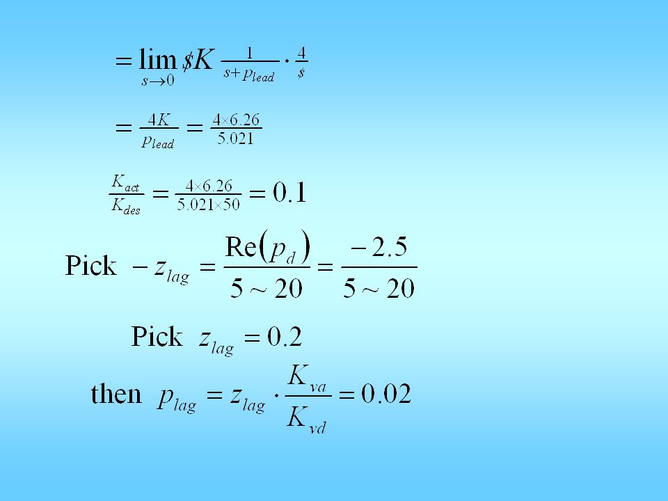
24. Use our formula to get p lead Now compute K : Now evaluate error constant K act

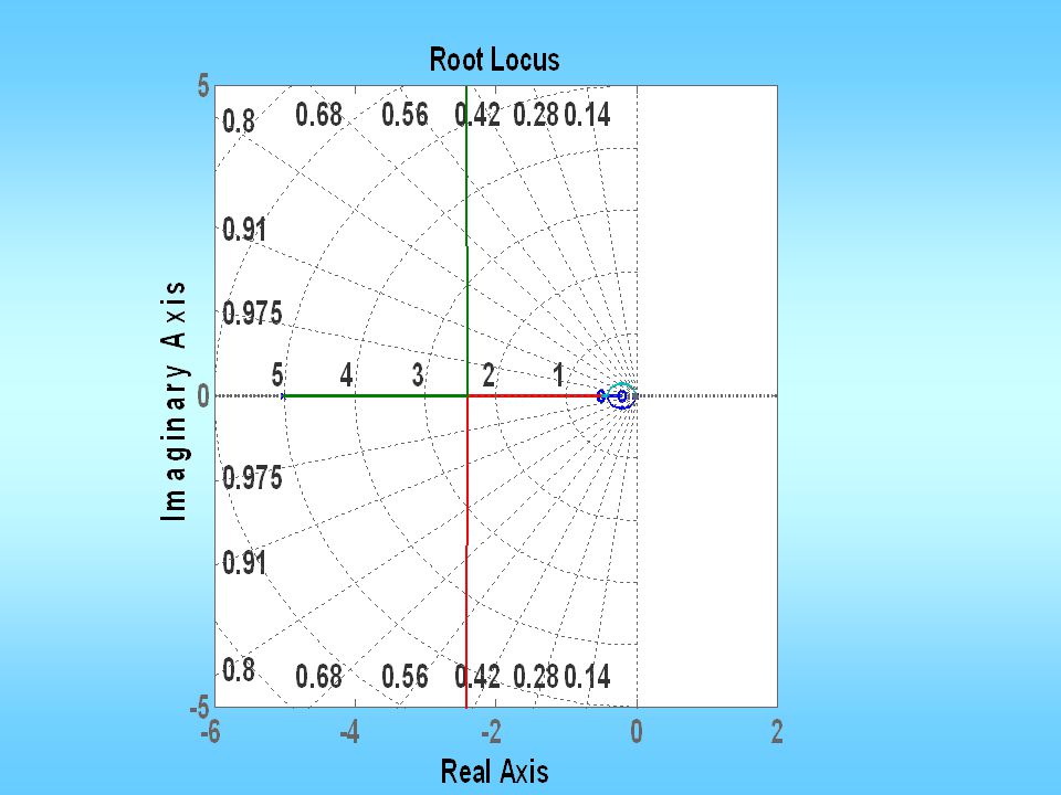
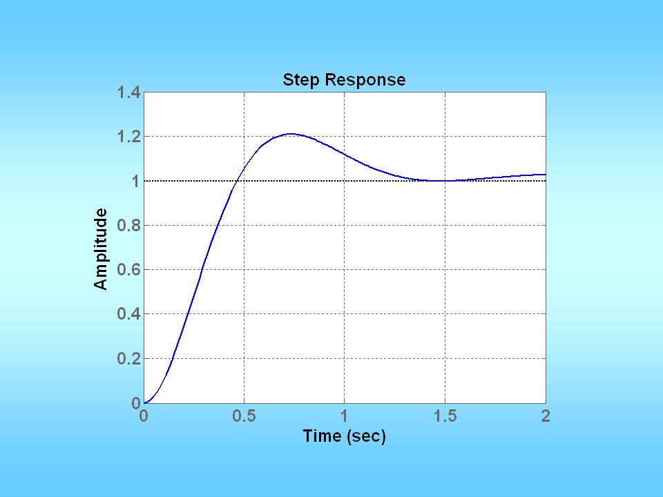
26. Could re-compute K, but let’s skip: do step response.

30. Lag control can improve e ss, but cannot totally eliminate e ss Use PI control to eliminate e ss PI :

31. PI Controller A PI controller can also be viewed as a Lag with p=0 PI controllers are used to get rid of a nonzero steady state error, by increasing the type by 1. It has strong destabilizing effects.

32. First PI design (a special Lag design): 1.Draw R.L. for G(s) 2.From specs, draw desired region 3.Pick p d on R.L. & in region 4.i. Choose ii. Choose 5. 6.Simulate & tune PI Design steps

33. Alternative PI design Since PI = PD/s, Can first multiply system by 1/s Then design using PD The overall controller is the controller you designed divided by s

34. Overall controller design 1.Draw R.L. for G(s), hold graph 2.Draw desired region for closed-loop poles based on desired specs 3.If R.L. goes through region, pick p d on R.L. and in region. Go to step 7. C(s)G p (s) R(s)E(s)Y(s)U(s)

35. 4.Pick p d in region (near corner but inside region for safety margin) 5.Compute angle deficiency: 6.a. PD control, choose z pd such that then

36. 6.b. Lead control: choose z lead, p lead such that You can select z lead & compute p lead. Or you can use the “bisection” method to compute z and p. Then If  < 60~70 deg, a single stage of PD or lead will work. If  > 80~90 deg, use a two-lead or PD-lead controller.

37. 7.Compute overall gain: 8.If there is no steady-state error requirement, go to 14. 9.With K from 7, evaluate error constant that you already have:

38. The 0, 1, 2 should match p, v, a This is for lag control. For PI:

39. 10.Compute desired error const. from specs: 11.For PI : set K * a = K * d & solve for z pi For lag : pick z lag & let

40. 12.Re-compute K (this step may be unnecessary) 13. 14.Get closed-loop T.F. Do step response analysis. 15.If not satisfactory, go back to 3 and redesign.

41. If we have both PI and PD we have PID control:

42. If we have both Lead and Lag, we have lead-lag control:

43. Control System Implementation C(s)G p (s) R(s)E(s)Y(s)U(s) ControllerActuator Reference Command error output control Plant Sensor disturbance input noise + _ plant input

44. PC-in-the-loop Control Power Amp Actuator Reference Command output Plant Sensor disturbance input A/D D/A PC I/O All control algorithms implemented in PC (could be Matlab Real-Time) Needs data acquisition system, including A/D and D/A Needs power amplifier Signal conditioner and amplifier

45.  -Controller based control Power Amp Actuator Reference Command output Plant Sensor disturbance input  -Controller I/O Very similar architecture to PC-in-the-loop control All control algorithms implemented in  -controller  -controller has its own A/D and D/A, but make sure resolution is OK Still needs power amplifier, because  -controller outputs weak signal Signal conditioner and amplifier

46. Power electronic based control Op Amp circuit Actuator Reference Command output Plant Sensor disturbance input Difference amplifier Analog operation, fastest Inexpensive All algorithms in circuit hardware Op Amp circuits for various controllers are given in book No sampling and aliasing issues