1. Three-dimensional tables (Please Read Chapter 3)

2. Analogy to factorial ANOVA, again Bacteria Type Temp123 Cool Warm Bacteria Type Temp123 Cool Warm Sweet potatoes White potatoes

3. Three Factors Storage temperature Bacteria type Potato type Dependent variable is amount of rot – mean rot in each cell. In log-linear models, there is no quantitative dependent variable.

4. Main effects Main effect for Temperature means, averaging over Bacteria Type and Potato Type, there is a difference in average rot between cool and warm storage. Main effect for Bacteria Type means, averaging over Temperature and Potato Type, there is a difference in average rot among the 3 types of bacteria. Main effect for Potato Type means, averaging over Bacteria Type and Temperature, there is a difference in average rot between sweet potatoes and white potatoes.

5. Two-factor interactions Bacteria Type by temperature interaction means that, averaging over potato type, the pattern of differences (in mean rot) among bacteria types depends on storage temperature. Or equivalently, the difference in mean rot between cool and warm temperature depends on bacteria type. Similar statements about potato type by Bacteria type and Potato type by Temperature.

6. 3-Factor Interaction The nature of the Bacteria Type by Temperature interaction depends on Type of Potato, or The nature of the Potato Type by Temperature interaction depends on Bacteria Type, or The nature of the Bacteria Type by Potato Type interaction depends on Temperature. All equivalent

7. Four Factors: A B C D Four (sets of) main effects: A, B, C, D AxB, AxC, AxD, BxC, BxD, CxD AxBxC, AxBxD, AxCxD, BxCxD AxBxCxD The 4-factor interaction means that the nature of each 3-factor interaction depends on the level of the remaining factor (all equivalent).

8. Log-linear model for a k-dimensional table Model for log of expected frequencies Looks like model for a k-factor ANOVA, with log expected frequency playing the role of the cell mean. Main effects represent departure from equal marginal probabilities Two-factor interactions represent relationship (association, lack of independence) between variables in two-dimensional marginal tables. Three-factor interaction means the nature of the relationship depends on the value of the 3d variable. Etc.

9. Log-linear model for a 3-dimensional table is the mean of all log expected frequencies. Main effects are deviations of the marginal means from the grand mean, etc. Effects add to zero over any subscript in parentheses.

10. We will stick to hierarchical models If a higher-order term is in the model, all lower-order terms involving those variables must be in the model too. Non-hierarchical models are useful at times, but interpretation can be very tricky.

11. Florida Prison Data 1.Prisoner’s Race (B-W) 2.Victim’s Race (B-W) 3.Death Penalty (Y-N)

12. Bracket Notation Represent variables by numbers, or maybe letters, like (VR, PR, DP) For each variable, enclose vars involving highest order interaction in brackets Main effects and lower order interactions are implied, because the models are hierarchical. For example, [PR VR] [VR DP] means Prisoner’s race and Victim’s race are related, and Victim’s race and Death penalty are related, but any relationship between Prisoner’s race and Death penalty comes from the other 2 relationships. This is a model of conditional independence.

13. [PR VR] [VR DP] = [1 2] [2 3] 1.Prisoner’s Race (B-W) 2.Victim’s Race (B-W) 3.Death Penalty (Y-N) Obtain estimated expected frequencies by maximum likelihood, test goodness of fit with X 2 or G 2, approximately chisquare if the model is true.

15. Conditional independence is Important! [1 2] [2 3] means that variables 1 and 2 are related and variables 2 and 3 are related, but any connection between 1 and 3 appears only because they are both related to 2. Given (that is, conditionally upon) the value of variable 2, Variables 1 and 3 are independent. Controlling for (allowing for) variable 2, there is no relationship between variables 1 and 3. Simpson’s paradox: Vars 1 and 3 seem to be related but looking at it separately for each level of Var 2, the relationship disappears or even reverses direction. Kidney stones: V1 = Treatment, V3=Effectiveness, V2=Size of stones.

16. It’s like multiple regression Suppose X 1 and X 2 are correlated, with Are X 1 and Y related? Yes!

17. But X 1 and Y are independent conditionally on the value of X 2 [X 1 X 2 ] [X 2 Y] “Controlling” for X 2, Y is unrelated to X 1

18. Iterative proportional model fitting Maximum likelihood estimation is indirect Go straight to estimation of expected frequencies First a example from the text: [1 2] [1 3] [2 3] Analytically, obtain

20. Try to make marginals match up. Update all cells at each step.

21. Now repeat the cycle

22. Keep repeating Ratios go to one, so the process converges (proved). Stop when you get close enough. It converges to the right answer (proved). Can be extended to any model. This is typical of mature maximum likelihood estimation; It’s usually not what you think.

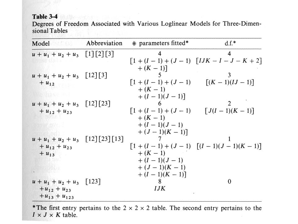
23. With expected frequencies, can test H 0 : Model is correct using df = Number of cells – Number of parameters in the model Look at Table 3-4 again

24. Getting the data into R Put frequencies directly into tables Read a data frame with frequencies, number of rows = number of cells Read a raw data file, number of rows = N

25. Put frequencies directly into tables For consistency with Table 3-5 in the text, make dimensions 1 = Perch Height, 2 = Perch Diameter, 3 = Species

27. Need Labels

28. Labels are dimnames of the array: A list

29. This is Better

30. Method 2: Read a data frame

31. Read data frame from an external file, say a plain text file in your working directory

32. Berkeley data are on the class website

33. xtabs(Counts ~ Vars separated by + signs, data = Name of data frame)

34. Marginal Tables are Easy Probably a data frame and xtabs is the easiest way to import data from a published table.

35. Method 3: External raw data file

36. Read data into a data frame, Number of rows = N

37. The table function

38. 3-Dimensional table

39. Fitting and testing models with the loglin function Hierarchical models only Very close to bracket notation Give it a table and a list of vectors Vectors are vars in a bracket, like c(1,2,4) means [1 2 4] Iterative proportional model fitting Returns estimated expected frequencies as an option

40. loglin(table,margin,fit=F,param=F)

42. Some options

43. Parameter estimates

44. Two more models: See right side of Table 3-5, p. 42