1. Spatial Analysis Grid cell counts

2. Grid Methods Data are recorded as coming from a particular area, but we do not have exact coordinates Screened artifacts from an excavation unit, census data (population counts from survey tracts, incidence of disease or other characteristic

3. Spatial Clusters Null hypothesis is that the data are distributed according to a Poisson distribution Variance/mean ratio (VMR) provides a rough indication of clustering where VMR = 1 is a Poisson distribution, 1 clustered

4. Visualizing Counts Choropleth maps represent quantity or category by shading polygons Dot density maps represent quantity/density by randomly or regularly spaced symbols within the polygon

5. Package sp Definitions for spatial objects SpatialPolygons are an object that contains a set of places (e.g. grid cells, states, counties) each of which can include multiple polygons and/or holes Perfect for choropleth and dot density maps

6. # Create a Spatial Polygons object source("GridUnits3a.R") # Append first line of coordinates to the bottom so # first-coord = last-coord Quads <- lapply(Quads, function(x) rbind(x, x[1,])) # Load package sp for spatial classes library(sp) # Create Polygon list (one from each unit) QuadsList <- lapply(Quads, function(x) Polygon(x, hole=FALSE)) # Areas3a <- sapply(QuadsList, function(x) x@area) to get areas # Create a Polygons list Units <- lapply(1:20, function(x) Polygons(QuadsList[x], UnitLbl[x])) # Create a Spatial Polygons list SPUnits <- SpatialPolygons(Units, 1:20) # sapply(1:20, function(x) SPUnits@polygons[[x]]@area) # to get areas from SpatialPolygons

7. opar <- par(mfrow=c(2, 2), mar=c(0, 0, 0, 0)) plot(SPUnits, col=gray(1:20/20)) plot(SPUnits, col=rainbow(20)) plot(SPUnits, col=rainbow(20, start=0, end=4/6)) plot(SPUnits, density=c(6:25), angle=c(45, -45)) plot(SPUnits, density=c(6:25), angle=c(-45, 45), add=TRUE) par(opar)

9. # Load FlkSize3a FlkDen3a <- round(sweep(FlkSize3a[,c("TCt", "TWgt")], 1, FlkSize3a$Area, "/"), 1) FlkDen3a <- data.frame(East=FlkSize3a$East, North=FlkSize3a$North, FlkDen3a) var(FlkDen3a$TCt)/mean(FlkDen3a$TCt) # Cut into 4 groups TCtGrp1 <- cut(FlkDen3a$TCt, quantile(FlkDen3a$TCt, c(0:4/4)), include.lowest=TRUE, dig=4) # TCtGrp2 <- cut(FlkDen3a$TCt, quantile(FlkDen3a$TCt, c(0:4/4)), # labels=1:4, include.lowest=TRUE) # TCtGrp3 <- cut(FlkDen3a$TCt, 0:4*1250+25, include.lowest=TRUE, # dig=4) Colors <- rev(rainbow(4, start=0, end=4/6)) Gray <- rev(gray(1:4/4)) Hatch <- c(5, 10, 15, 20)

10. opar <- par(mfrow=c(2, 2), mar=c(0, 0, 0, 0)) plot(SPUnits, col=Colors[as.numeric(TCtGrp1)]) text(985, 1015.75, "Total Flakes", cex=1.25) legend(985.5, 1022, levels(TCtGrp1), fill=Colors) plot(SPUnits, col=Gray[as.numeric(TCtGrp1)]) text(985, 1015.75, "Total Flakes", cex=1.25) legend(985.5, 1022, levels(TCtGrp1), fill=Gray) plot(SPUnits, angle=45, density=Hatch[as.numeric(TCtGrp1)]) plot(SPUnits, angle=-45, density=Hatch[as.numeric(TCtGrp1)], add=TRUE) text(985, 1015.75, "Total Flakes", cex=1.25) legend(985.5, 1022, levels(TCtGrp1), angle=45, density=Hatch) legend(985.5, 1022, levels(TCtGrp1), angle=-45, density=Hatch) par(opar)

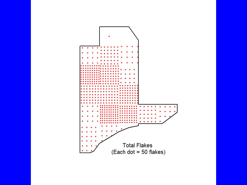
12. library(maptools) opar <- par(mfrow=c(2, 2), mar=c(0, 0, 0, 0)) for (i in 1:4) { dots <- dotsInPolys(SPUnits, as.integer(round(FlkDen3a$TCt/50, 0))) # 1 dot = 50 flakes plot(SPUnits, lty=0) points(dots, pch=20, col="red") polygon(c(982,982,983,983,984.5,985,985,987,987,986.2,985,985, 984.5,984,983.5,983,982.7,982.5),c(1015.5,1021,1021,1022, 1022,1021.3,1018,1018,1017.6,1017,1017,1016.9,1016.8,1016.6, 1016.3,1016,1015.6,1015.5), lwd=2, border="black") } par(opar) dots <- dotsInPolys(SPUnits, as.integer(round(FlkDen3a$TCt/50, 0)), f="regular") plot(SPUnits, lty=0) points(dots, pch=20, cex=.75, col="red") polygon(c(982,982,983,983,984.5,985,985,987,987,986.2,985,985,984.5, 984,983.5,983,982.7,982.5),c(1015.5,1021,1021,1022,1022,1021.3, 1018,1018,1017.6,1017,1017,1016.9,1016.8,1016.6,1016.3, 1016,1015.6,1015.5), lwd=2, border="black") text(985, 1015.75, "Total Flakes \n(Each dot = 50 flakes)", cex=1.25)

15. Countour Mapping We fit a model to the data to interpolate between the observations and smooth them –Trend surface models with polynomials –Kriging – developed in geophysics to interpolate and extrapolate

16. library(geoR) # load FlkDen3a.RData FlkDen3a$East <- FlkDen3a$East +.5 FlkDen3a$North <- FlkDen3a$North +.5 FlkDen3a$AvWgt <- FlkDen3a$TWgt/FlkDen3a$TCt columns <- names(FlkDen3a) Flakes3a <- as.geodata(FlkDen3a, 1:2, 3:5, c("TCt", "TWgt", "AvWgt")) GridPts <- expand.grid(East=seq(982, 987,.25), North=seq(1015.5, 1022,.25)) Border3a <- cbind(c(982,982,983,983,984.5,985,985,987,987,986.2, 985,985,984.5,984,983.5,983,982.7,982.5),c(1015.5,1021,1021, 1022,1022,1021.3,1018,1018,1017.6,1017,1017,1016.9,1016.8, 1016.6,1016.3,1016,1015.6,1015.5)) V <- variog(Flakes3a, data=Flakes3a$data[,"TCt"]) plot(V, type="b") vf <- variofit(V) TCtKv <- krige.conv(Flakes3a, data=Flakes3a$data[,"TCt"], locations=GridPts, krige=krige.control(cov.pars=c(1292000,.824))) contour(TCtKv, borders=Border3a, xlab="East", ylab="North") contour(TCtKv, borders=Border3a, axes=FALSE) contour(TCtKv, borders=Border3a, filled=TRUE) persp(TCtKv, borders=Border3a, xlab="East", ylab="North", zlab="Total Flakes", expand=.5)

20. Unconstrained Clustering Proposed by Robert Whallon Take grid data and computer percentages (areas defined by relative abundance, not density) Cluster grids and plot the distribution of the clusters to identify activity areas