Download presentation
Presentation is loading. Please wait.

1
Next

2
MS E XCEL 2007 The Microsoft Excel is on of the Microsoft Office suite of programs. Its primary function is to perform calculations, analyze information and manage lists spreadsheet. To start MS Excel 2007 using the Windows Start Menu Click Start All Programs Microsoft office Microsoft Excel 2007. Next

3
How to open MS Excel 2007

4
W ELCOME T O MS E XCEL !! Next

5
T HE MS E XCEL SCREEN ELEMENTS Title bar Menu bar Tool bar Cell Reference Formula bar Active cell Row Column Next

6
T HE E LEMENTS OF E XCEL W INDOW Element (part) Job المصطلح بالعربية Title bar Shows the name of the book شريط القوائم Menu bar Provides access to the commands on the menus شريط الأدوات Tool bar Standard toolbar: contains buttons to help you select common commands, such as save, open, undo typing and print. Formatting toolbar: contains buttons to help you select formatting commands, such as font size, font style, bold alignment and font color. جزء المهام Row A horizontal line of cells. صف Column A vertical line of cells. عامود Active cell Display a thick border. You enter data into the active cell. الخلية النشيطة Cell reference (Name box) A cell’s address. For example, the cell at the intersection of column A and row 1 has the reference A1. عنوان الخلية Formula bar Allows you to calculate and analyze data or change information in a worksheet. شريط الصيغة الرياضية Row heading A number identifies each row. عنوان صف Column heading A letter identifies each column. عنوان عامود
 A cell’s address. For example, the cell at the intersection of column A and row 1 has the reference A1. عنوان الخلية Formula bar Allows you to calculate and analyze data or change information in a worksheet. شريط الصيغة الرياضية Row heading A number identifies each row. عنوان صف Column heading A letter identifies each column. عنوان عامود.")
7
E NTER D ATA : Enter numbers in a cell. - Select the cell in which you want to enter a number and type in the number. - The number you type appears in the active cell and the formula bar. - Press the Enter Key to enter the number and move down one cell. - If you want to make the number a negative, type a minus sign in front it or enclose it in parentheses (i.e. brackets). - The numbers will be right aligned by default. Enter text in a cell. - Click the cell where you want to enter text. Then type the text. - The text you type appears in the active cell and the formula bar. - Remember that to move to the next cell use the Tab Key. - To move down a cell press the Enter Key. he text will be left aligned by default. N e x t
. - The numbers will be right aligned by default. Enter text in a cell. - Click the cell where you want to enter text. Then type the text. - The text you type appears in the active cell and the formula bar. - Remember that to move to the next cell use the Tab Key. - To move down a cell press the Enter Key. he text will be left aligned by default. N e x t.")
9
E NTER S YMBOLS OR S PECIAL C HARACTERS IN A C ELL. - Select the Symbol command from the Insert menu.

10
S ELECT C ELL Select a cell - Click the cell you want to select. - The cell becomes an active cell and displays a thick border. Select a row(s) - Click the number of the row (Row Heading) you want to select - To select multiple rows, position the mouse over the number of the first row you want to select. Then drag the mouse until you highlight all the rows you want to select. Next
 - Click the number of the row (Row Heading) you want to select - To select multiple rows, position the mouse over the number of the first row you want to select. Then drag the mouse until you highlight all the rows you want to select. Next.")
11
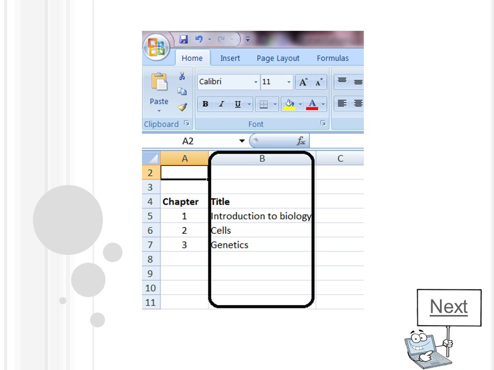
Select a column(s) - Click the number of the column (Column Heading) you want to select. - To select multiple columns, position the mouse over the letter of the first column you want to select. Then drag the mouse until you highlight all the columns you want to select. Select a group of cells -Position the mouse over the first cell you want to select. - Drag the mouse until you highlight all the cells you want to select. Next

12
Select non-adjacent cells. - Click on the first cell you wish to select. Depress the Control Key (Ctrl). - Click on the other cell you wish to select. Release the Control key when you have finished. Complete a series Excel can save you time by completing a text or number series for you. Complete a Text Series. - Enter the text you want to start the series. - Click the cell containing the text you entered. - Position the mouse over the bottom right corner of the cell, (Auto Fill Hand). - Drag the mouse + over the cells you want to include in the series. - The cells display the text series. Auto Fill Hand
. - Click on the other cell you wish to select. Release the Control key when you have finished. Complete a series Excel can save you time by completing a text or number series for you. Complete a Text Series. - Enter the text you want to start the series. - Click the cell containing the text you entered. - Position the mouse over the bottom right corner of the cell, (Auto Fill Hand). - Drag the mouse + over the cells you want to include in the series. - The cells display the text series. Auto Fill Hand.")
13
Complete a Number Series. - Enter the first two numbers you want to start the series. - Click the cells containing the numbers you entered. - Position the mouse over the bottom right corner of the cells, (Auto Fill Hand). - Drag the mouse + over the cells you want to include in the series. - The cells display the number series. Auto Fill Hand Next
. - Drag the mouse + over the cells you want to include in the series. - The cells display the number series. Auto Fill Hand Next.")
14
Copy, Move, Delete Use the copy and paste tools to duplicate cell contents in another part of a worksheet. -Select the cell or range you wish to copy. -From the edit menu select copy. or press Ctrl+C, or right click on the mouse select copy or click on the copy icon on the standard toolbar. -Switch to the required destination program. -Place the cursor where you want the data to appear. -select paste from the edit menu or press Ctrl+V or right click on the mouse select copy or select the paste icon from the standard toolbar. Delete cell contents in a selected cell range. -Select the cell or range that you want to delete. -From the edit menu select delete.

15
Search and replace Use the search command for specified cell content. -Place the insertion point where you want to begin the search. -Select the find command from the edit menu. or press Ctrl+F to display the find dialog box.

16
UUse the replace command from the edit menu. or press Ctrl+H to display the replace dialog box.

17
Rows and Columns To insert a row into worksheet. -Excel will insert a row above the row you select. (to select a row, click the row number). -To select more than one row, drag the mouse pointer across the required row headings (with mouse button depressed). -Click insert menu Rows. Or right click over the selected row(s) to display a pop-up menu, select insert. 2.Insert a row 1.Select a row
. -To select more than one row, drag the mouse pointer across the required row headings (with mouse button depressed). -Click insert menu Rows. Or right click over the selected row(s) to display a pop-up menu, select insert. 2.Insert a row 1.Select a row.")
18
The new row appears and all rows that follow shift downward. Next

19
To insert a column into worksheet -Excel will insert a column to the left of the column you select. (To select a column, click the column letter). -To select more than one column, drag the mouse pointer across the required column headings (with mouse button depressed). -Click insert menu columns Or right click over the selected columns(s) to display a pop-up menu, select insert. 1.Insert a column 2.Select a column Next
. -To select more than one column, drag the mouse pointer across the required column headings (with mouse button depressed). -Click insert menu columns Or right click over the selected columns(s) to display a pop-up menu, select insert. 1.Insert a column 2.Select a column Next.")
20
The new column appears and all the columns that follow shift to the right. Next

21
Modify column width and row height TTo change the width of a column -Position the mouse Over the right edge of the column heading. - Drag the column edge until the dotted line displays the column width you want. -Fit longest itemTo Change a column width to fit the longest item in the column, double-click the right edge of the column heading. Next

23
To change the height of a row -Position the mouse Over the bottom edge of the row heading. - Drag the row edge until the dotted line displays the row height you want. - Fit tallest itemTo change a row height to fit the tallest item in the row-double-click the bottom edge of the row heading.

24
Insert a worksheet You can insert a new worksheet to add related data to your workbook. Each workbook you create automatically contains three worksheets. You can insert as many new worksheets as you need. Click insert worksheet First step Next

25
Second step Third step The new worksheet appears

26
Delete a worksheet You can permanently remove a worksheet you no longer need from your workbook. Right-click the tab of worksheet you want to delete select delete. Or click edit Delete sheet

27
R ENAME A WORKSHEET - Right click on the worksheet tab that you wish to rename. From the popup menu Displayed select the Rename command. - You can then type over the default worksheet name, which will become highlighted.

28
Change font of Data -Select the cells containing the data you want to a new font -Click in this area to display the list of the available fonts. -Click the font you want to use -The data changes to the font you selected. Next

30
Change size of Data -Select the cells containing the data you want to a new size. -Click in this area to display a list of the available sizes. -Click the size you want to use. Next

32
Change cell color (Cell Shading). -Select the cells you want to change to a different color. -Click in this area to select a color from the Toolbar. -Click the color you want to use Next

33
To remove a color from Cells, repeat steps 1to 3, Except select No Fill in step 3 Next

34
Change Data Color. -Select the cells containing the data you want to different color -Click in this area to select a color from the Toolbar -Click the color you want to use Next

35
To remove a color from Cells, repeat steps 1to 3, Except select Automatic in step 3 Next

36
BBold, Italic, Underline - Select the cells containing the data you want to change -Click one of the following buttons from the Toolbar. BoldUnderlineItalic CChange alignment of Data -Select the cells containing the data you want to align differently -Click one of the following buttons from the Toolbar. Align leftCenterAlign right Bold, Underline, Center, Font Size12 points, Font color red Bold, Italic, Align Left, Font Size 10 points Next

37
CHANGE NUMBER FORMAT CChange the number styles -Select the cells containing the number you want to change -Click one of the following buttons from the Toolbar. CurrencyComma AAdd or remove a Decimal Place -Select the cells containing the number you want to change -Click one of the following buttons from the Toolbar. Percent IncreaseDecrease Next

38
-Enter a number in a cell -Right Click to display a pop-up menu, and select Format Cells, to display the format cells dialog box -Select Number, Currency, or Percentage from the category list.

39
Currency (dollar value) Decimal Places
 Decimal Places")
42
Returns the average (arithmetic mean) of the arguments. Example : (find the average for each student.)
.")
43
A dialog box appears. If the dialog box covers data you want to use in calculations, you can move the dialog box to a new location

44
Returns the average (arithmetic mean) of the arguments. Example : (find the Average for each student.)
.")
45
SyntaxDefinitionFunction Name MAX(number1, number2,…) Number1, number2, … are 1 to 30 numbers for which you want to find the maximum value. Returns the largest value in a set of values. Max MIN(number1,number2,…) Number1, number2,… are 1 to 30 numbers for which you want to find the minimum value. Returns the smallest number in a set of values. Min Sum(number1, number2,…) Number1, number2, … are 1 to 30 arguments for which you want the total value or sum. Adds all the numbers in a range of cells. Sum Average(number1, number2,…) Number1, number2, … are 1 to 30 numeric arguments for which you want the average. Returns the average (arithmetic mean) of the arguments. Average COUNT(value1, value2,…) Value 1, value2,… are 1 to 30 arguments that can contain or refer to a variety of different types of data, but only numbers are counted. Counts the numbers of cells that contain numbers and counts numbers within the list of arguments.Use COUNT to get the number of entries in a number field that is in a range or array of numbers. Count COUNTA(value1, value2,…) Value1,value2,… are 1 to 30 arguments representing the values you want to count. Counts the number of cells that are not empty and the values within the list of arguments. Use COUNTA to count the number of cells that contain data in a range or array. Count A COUNTBLANK(range) Range is the range from which you want to count the blank cells Counts empty cells in a specified range of cells CountBlank
 Number1, number2,… are 1 to 30 numbers for which you want to find the minimum value. Returns the smallest number in a set of values. Min Sum(number1, number2,…) Number1, number2, … are 1 to 30 arguments for which you want the total value or sum. Adds all the numbers in a range of cells. Sum Average(number1, number2,…) Number1, number2, … are 1 to 30 numeric arguments for which you want the average. Returns the average (arithmetic mean) of the arguments. Average COUNT(value1, value2,…) Value 1, value2,… are 1 to 30 arguments that can contain or refer to a variety of different types of data, but only numbers are counted. Counts the numbers of cells that contain numbers and counts numbers within the list of arguments.Use COUNT to get the number of entries in a number field that is in a range or array of numbers. Count COUNTA(value1, value2,…) Value1,value2,… are 1 to 30 arguments representing the values you want to count. Counts the number of cells that are not empty and the values within the list of arguments. Use COUNTA to count the number of cells that contain data in a range or array. Count A COUNTBLANK(range) Range is the range from which you want to count the blank cells Counts empty cells in a specified range of cells CountBlank.")
51
The End

Similar presentations


. Is a spreadsheet application designed to take advantage of the windows graphical interface MICROSOFT EXCEL.>")


 Excel Lessons 1, 2 and 3 Press Space bar to Advance Frame.>")


>")