Download presentation
Presentation is loading. Please wait.

1
Chapter 7 Statistical Data Treatment and Evaluation
Experimentalist use statistical calculations to sharpen their judgments concerning the quality of experimental measurements. These applications include: Defining a numerical interval around the mean of a set of replicate analytical results within which the population mean can be expected to lie with a certain probability. This interval is called the confidence interval (CI).
.")
2
Determining the number of replicate measurements required to ensure at a given probability that an experimental mean falls within a certain confidence interval. Estimating the probability that (a) an experimental mean and a true value or (b) two experimental means are different. Deciding whether what appears to be an outlier in a set of replicate measurements is the result of a gross error or it is a legitimate result. Using the least-squares method for constructing calibration curves.
 an experimental mean and a true value or (b) two experimental means are different. Deciding whether what appears to be an outlier in a set of replicate measurements is the result of a gross error or it is a legitimate result. Using the least-squares method for constructing calibration curves.")
3
Finding the Confidence Interval when s Is a Good Estimate of
CONFINENCE LIMITS Confidence limits define a numerical interval around x that contains with a certain probability. A confidence interval is the numerical magnitude of the confidence limit. The size of the confidence interval, which is computed from the sample standard deviation, depends on how accurately we know s, how close standard deviation is to the population standard deviation . Finding the Confidence Interval when s Is a Good Estimate of A general expression for the confidence limits (CL) of a single measurement CL = x z For the mean of N measurements, the standard error of the mean, /N is used in place of CL for = x z/N _ _ _
 of a single measurement. CL = x z For the mean of N measurements, the standard error of the mean, /N is used in place of CL for = x z/N. _. _. _.")
5
Finding the Confidence Interval when Is Unknown
We are faced with limitations in time or the amount of available sample that prevent us from accurately estimating . In such cases, a single set of replicate measurements must provide not only a mean but also an estimate of precision. s calculated from a small set of data may be quite uncertain. Thus, confidence limits are necessarily broader when a good estimate of is not available.

6
…continued… To account for the variability of s, we use the important statistical parameter t, which is defined in the same way as z except that s is substituted for . t = (x - ) / s t depends on the desired confidence level, but t also depends on the number of degrees of freedom in the calculation of s. t approaches z as the number of degrees of freedom approaches infinity. The confidence limits for the mean x of N replicate measurements can be calculated from t by an equation CL for = x ts/N _ _
 / s. t depends on the desired confidence level, but t also depends on the number of degrees of freedom in the calculation of s. t approaches z as the number of degrees of freedom approaches infinity. The confidence limits for the mean x of N replicate measurements can be calculated from t by an equation. CL for = x ts/N. _. _.")
8
Comparing an Experimental Mean with the True Value
A common way of testing for bias in an analytical method is to use the method to analyze a sample whose composition is accurately known. Bias in an analytical method is illustrated by the two curves shown in Fig. 7-3, which show the frequency distribution of replicate results in the analysis of identical samples by two analytical methods. Method A has no bias, so the population mean A is the true value xt. Method B has a systematic error, or bias, that is given by bias = B - xt = B - A bias effects all the data in the set in the same way and that it can be either positive or negative.

10
The critical value for rejecting the null hypothesis is calculated by
…continued… The difference x – xt is compared with the difference that could be caused by random error. If the observed difference is less than that computed for a chosen probability level, the null hypothesis that x and xt are the same cannot be rejected. It says only that whatever systematic error is present is so small that it cannot be distinguished from random error. If x –xt is significantly larger than either the expected or the critical value, we may assume that the difference is real and that the systematic error is significant. The critical value for rejecting the null hypothesis is calculated by x – xt= ts /N _ _ _ _

11
Comparing Two Experimental Means
The results of chemical analyses are frequently used to determine whether two materials are identical. The chemist must judge whether a difference in the means of two sets of identical analyses is real and constitutes evidence that the samples are different or whether the discrepancy is simply a consequence of random errors in the two sets. Let us assume that N1 replicate analyses of material 1 yielded a mean value of x1 and that N2 analyses of material 2 obtained by the same method gave a mean of x2. If the data were collected in an identical way, it is usually safe to assume that the standard deviations of two sets of measurements are the same. We invoke the null hypothesis that the samples are identical and that the observed difference in the results, (x1 – x2), is the result of random errors. _ _ _ _
, is the result of random errors. _. _. _. _.")
12
The standard deviation of the mean x1 is
…continued… The standard deviation of the mean x1 is and like wise for x2, Thus, the variance s2d of the difference (d = x1 – x2) between the means is given by s2d = s2m1 + s2m2 _ _ _ _
 between the means is given by. s2d = s2m1 + s2m2. _. _. _. _.")
13
…continued… By substituting the values of sd, sm1, and sm2 into this equation, we have If we then assume that the pooled standard deviation spooled is a good estimate of both sm1 and sm2, then and 2 2 2 2 2 2 2 1/2

14
Substituting this equation, we find that
or the test value of t is given by We then compare our test value of t with the critical value obtained from the table for the particular confidence level desired. If the absolute value of the test statistic is smaller than the critical value, the null hypothesis is accepted and no significant difference between the means has been demonstrated. A test value of t greater than the critical value of t indicates that there is a significant difference between the means. _ _ _ _

15
DETECTING GROSS ERRORS
A data point that differs excessively from the mean in a data set is termed an outlier. When a set of data contains an outlier, the decision must be made whether to retain or reject it. The choice of criterion for the rejection of a suspected result has its perils. If we set a stringent standard that makes the rejection of a questionable measurement difficult, we run the risk of retaining results that are spurious and have an inordinate effect on the mean of the data. If we set lenient limits on precision and thereby make the rejection of a result easy, we are likely to discard measurements that rightfully belong in the set, thus introducing a bias to the data. No universal rule can be invoked to settle the question of retention or rejection.

16
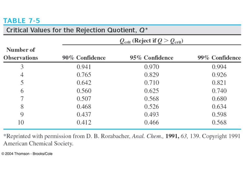
Using the Q Test The Q test is a simple and widely used statistical test. In this test, the absolute value of the difference between the questionable result xq and its nearest neighbor xn is divided by the spread w of the entire set to give the quantity Qexp: This ratio is then compared with rejection values Qcrit found in Table. If Qexp is greater the Qcrit, the questionable result can be rejected with the indicated degree of confidence.

19
How Do We Deal with Outliers?
Reexamine carefully all data relating to the outlying result to see if a gross error could have affected its value. If possible, estimate the precision that can be reasonably expected from the procedure to be sure that the outlying result actually is questionable. Repeat the analysis if sufficient sample and time are available. If more data cannot be obtained, apply the Q test to the existing set to see if the doubtful result should be retained or rejected on statistical grounds. If the Q test indicates retention, consider reporting the median of the set rather than the mean.

20
ANALYZING TWO-DIMENSIONAL DATA: THE LEAST-SQUARES METHOD
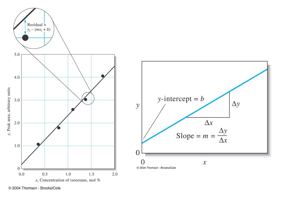
Many analytical methods are based on a calibration curve in which a measured quantity y is plotted as a function of the known concentration x of a series of standards. The typical calibration curve shown in Fig The ordinate is the dependent variable and the abscissa is the independent variable. As is typical (and desirable), the plot approximates a straight line. However, because of the indeterminate errors in the measurement process, not all the data fall exactly on the line. Thus, the investigator must try to draw the “best” straight line among the points. A statistical technique called regression analysis provides the means for objectively obtaining such a line and also for specifying the uncertainties associated with its subsequent use.
, the plot approximates a straight line. However, because of the indeterminate errors in the measurement process, not all the data fall exactly on the line. Thus, the investigator must try to draw the best straight line among the points. A statistical technique called regression analysis provides the means for objectively obtaining such a line and also for specifying the uncertainties associated with its subsequent use.")
22
Assumptions of the Least-Squares Method
When the method of least squares is used to generate a calibration curve, two assumptions are required. The first is the there is actually a linear relationship between the measured variable (y) and the analyte concentration (x). The mathematical relationship that describes this assumption is called the regression model, which may be represented as y = mx + b where, b is the y intercept (value of y when x is zero) and m is the slope of the line. We also assume that deviation of individual points from the straight line results from error in the measurement. That is, we must assume that there is no error in the x values of the points. We assume that exact concentrations of the standards are known. Both of these assumption are appropriate for many analytical methods.
 and the analyte concentration (x). The mathematical relationship that describes this assumption is called the regression model, which may be represented as. y = mx + b. where, b is the y intercept (value of y when x is zero) and m is the slope of the line. We also assume that deviation of individual points from the straight line results from error in the measurement. That is, we must assume that there is no error in the x values of the points. We assume that exact concentrations of the standards are known. Both of these assumption are appropriate for many analytical methods.")
23
Computing the Regression Coefficients and Finding the Least-Squares Line
The vertical deviation of each point from the straight line is called a residual. The line generated by the least-squares method is the one that minimizes the sum of the squares of the residuals for all the points. In addition to providing the best fit between the experimental points and the straight line, the method gives the standard deviations for m and b.

24
We define three quantities Sxx, Syy, and Sxy as follows:
…continued… We define three quantities Sxx, Syy, and Sxy as follows: Sxx = (xi – x)2 = x2i – (xi)2 / N Syy = (yi – y)2 = y2i – (yi)2 / N Sxy = (xi – x)(yi – y) = xiyi– [(xiyi)] / N where, xi and yi are individual pairs of data for x and y, N is the number of pairs of data used in preparing the calibration curve, and x and y are the average values for the variables; that is, x = xi / N and y = yi / N
2 = x2i – (xi)2 / N. Syy = (yi – y)2 = y2i – (yi)2 / N. Sxy = (xi – x)(yi – y) = xiyi– [(xiyi)] / N. where, xi and yi are individual pairs of data for x and y, N is the number of pairs of data used in preparing the calibration curve, and x and y are the average values for the variables; that is, x = xi / N and. y = yi / N.")
Similar presentations


>")


