Review: Correlation vs. Regression  What are the main differences between correlation & regression?  What are the data requirements for each?  What.

Review: Correlation vs. Regression  What are the main differences between correlation & regression?  What are the data requirements for each?  What are their principal vulnerabilities?  How do we establish causality?

 Pearson correlation: a linear association between two quantitative variables.

Data Requirements  A probability sample—if the analysis will be inferential, as opposed to descriptive.  For OLS regression, the outcome variable must be quantitative (interval or ratio); the explanatory variables may be quantitative or categorical (nominal or ordinal).

 What are the disadvantages of using correlation to study the relationships between two or more variables?  See Moore/McCabe, chapter 2.

Hypothesis tests for correlation  We can use Pearson correlation not only descriptively but also inferentially.  To use it inferentially, use a scatterplot to check the bivariate relationship for linearity.  If the relationship is sufficiently linear:

In Stata, ‘pwcorr’ vs. ‘corr’  ‘correlate’ (corr): ‘listwise,’ or ‘casewise,’ deletion— i.e. any observation (i.e. individual, case) for which any of the correlated variables has missing data is not used (i.e. ‘corr’ only uses observations with complete data for the examined variables).  If, for the relationship between math and reading scores, observation #27 has, say, a missing math score, then ‘corr’ or ‘regress’ will automatically drop observation #27.  This is how regression works, so ‘corr’ corresponds to regression.  Moreover, ‘corr’ does not permit hypothesis tests.

 pwcorr: (‘pairwise’) uses all of the non-missing observations for the examined variables (e.g., it would use observation #27’s reading score, even though #27’s math score is missing).  This does not correspond to the way that regression works.  Moreover, pwcorr permits hypothesis tests  Note: There is a way to use ‘pwcorr’ so that, like regression analysis, it is based on casewise (i.e. listwise) deletion of missing observations. We’ll demonstrate this later.

 Use a Bonferonni or other multiple- test adjustment when simultaneously testing multiple correlation hypotheses:. pwcorr read write math science socst, obs sig star(.05) bonf  Why is the multiple-test adjustment important?

 If the data have no missing values, then there’s no problem using pwcorr.

Contingency Table vs. Pearson Correlation  What if the premises of parametric statistics don’t hold?  E.g., what if the quantitative variables are based on a small sample (say, <30)?  Or what if the relationship is non-linear, and possible transformations (such as logarithmic) aren’t applicable or don’t work, and/or it doesn’t make sense to eliminate extreme outliers?  What if the quantitative variables are ordinal rather than interval in measurement?

 In such cases it may be useful to: (1) use non-parametric procedures (such as Spearman rho [in Stata: ‘spearman x y’]); or (2) categorize the data & assess the bivariate association via a contingency table.  Non-parametric procedures are not premised on the approximate normality of the sample distribution of sample means (see the Moore/McCabe chap. 7 & CD-Rom chapter).  As for contingency tables, here’s an example of how to do a contingency table in response to violated parametric assumptions: What’s the association between science & reading scores?

. xtile xsci=science, nq(4). xtile xread=read, nq(4). tab1 xsci xread. bys xsci: su science. bys xread: su read. tab xread xsci, col chi2  Always have a good reason for how you categorize a quantitative variable.  Check # observations per cell for the validity of the Chi-square hypothesis test.

Measures of Correlation & Association Involving Categorical Variables  Here are some alternatives to Pearson correlation (including nonparametric [‘rank’] statistics):

There are other correlation coefficients & measures of association (besides ttest & prtest) for categorical variables & for combinations of categorical & continuous variables. E.g.:  Spearman correlation (i.e. ‘rank correlation’; see Moore/McCabe chap. 7 and CD-Rom chapter, Hamilton, chap. 6 & Stata Manual) (It is also an outlier-resistant alternative to ‘corr’ or ‘pwcorr’ for quantitative variables.):. spearman ordinalscore ses  Kendall’s tau (like Spearman, but can be slower in Stata; see Hamilton, chap. 6 & Stata Manual). ktau ordinalscore ses

 eta-squared: when one variable is quantitative continuous & the other is multi-level categorical (see Moore/McCabe, chap. 12, ‘ANOVA’; Hamilton, chap. 5, ‘ANOVA’; Stata Manual, ‘oneway’).. oneway read ses, tabulate bonf [Bartlett test must be insignificant; see also ANOVA and loneway.]  biserial correlation & point biserial correlation: when one variable is quantitative continuous & the other is binary. Just use ‘corr’ or ‘pwcorr’—Stata or any other major software automatically makes the adjustment:. pwcorr read female, obs sig star(.05) [same result as ttest read,by(female)]

 phi coefficient: two categorical binary variables.. pwcorr female white, obs sig star(.05) [same result as tab female white, col/row/cell chi2]. tab female ses, all [output includes ‘Cramer’s V,’ which is an adaptation of phi coefficient for tables that are larger than two-by-two, but it likewise works in two-by-two tables]  Caution: Recall the ramifications of restricted-range data and ecological data for correlation results, & recall the need to consider lurking variables.

 Non-parametric: rank data.  Parametric: premised on approximately normal sampling distribution of sample means (i.e. Central Limit Theorem).

CI’s for Pearson & Spearman correlations:. findit ci2 [& download]. ci2 read write, corr Confidence interval for Pearson's product-moment correlation of read and write, based on Fisher's transformation. Correlation = 0.597 on 200 observations (95% CI: 0.499 to 0.679). ci2 read ses, corr spearman Confidence interval for Spearman's rank correlation of read and ses, based on Fisher's transformation. Correlation = 0.280 on 200 observations (95% CI: 0.147 to 0.403)

Regression Analysis

 What are regression analysis’s major advantages over the alternatives for examining the relationships between two or more variables (see Moore/McCabe, chapter 2)?  Regression: examines how the values of an outcome variable y depend on the values of one or more explanatory variables x (i.e. the slope & direction of the y/x straight line).

 On average, how does risk of heart disease (y) change with every unit of increase or decrease in amount of fat consumption (x 1 ) & in amount of exercise (x 2 )?  On average, how does earnings level (y) change with every unit of increase or decrease in years of education (x 2 ) & in years of person’s age (x 1 )?

 Recall the problems of causality that we discussed in Chapter Two.  Always ask: What is the conceptual basis of the hypothesized or implied causal relationship? What if it were reversed?  See, e.g., King et al., Designing Social Inquiry; McClendon, Multiple Regression and Causal Analysis; Berk, Regression Analysis: A Constructive Critique.

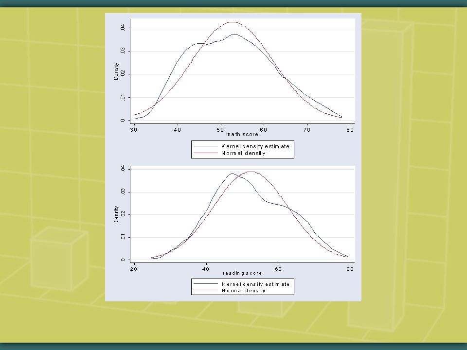
 Let’s start by interpreting the following simple regression model (i.e. regression model with one explanatory variable x).  use hsb2, clear. for varlist math read: kdensity X, norm \ more

. gr box math read

. su math read, d math score ------------------------------------------------------------- Percentiles Smallest 1% 36 33 5% 39 35 10% 40 37 Obs 200 25% 45 38 Sum of Wgt. 200 50% 52 Mean 52.645 Largest Std. Dev. 9.368448 75% 59 72 90% 65.5 73 Variance 87.76781 95% 70.5 75 Skewness.2844115 99% 74 75 Kurtosis 2.337319 reading score ------------------------------------------------------------- Percentiles Smallest 1% 32.5 28 5% 36 31 10% 39 34 Obs 200 25% 44 34 Sum of Wgt. 200 50% 50 Mean 52.23 Largest Std. Dev. 10.25294 75% 60 73 90% 67 73 Variance 105.1227 95% 68 76 Skewness.1948373 99% 74.5 76 Kurtosis 2.363052

. scatter math read || qfit math read

. corr math read (obs=200) | math read ---------+------------------ math | 1.0000 read | 0.6623 1.0000. pwcorr math read, obs sig | math read -------------+------------------ math | 1.0000 | | 200 | read | 0.6623 1.0000 | 0.0000 | 200 200

. reg math read SourceSS df MS Number of obs = 200 F( 1, 198) = 154.70 Model7660.75905 1 7660.75905 Prob > F= 0.0000 Residual9805.03595 198 49.5203836 R-squared= 0.4386 Adj R-squared = 0.4358 Total17465.795 199 87.7678141 Root MSE= 7.0371 mathCoef.Std. Err. tP>t[95% Conf.Interval] read.6051473.0486538 12.440.000.509201.7010935 _cons21.038162.58945 8.120.00015.93172 26.1446  Interpretation?

 The simple linear regression model assumes that the mean of the outcome variable is a linear function of one explanatory variable.  The multiple linear regression model—as we’ll later see—assumes that the mean of the outcome variable is a linear function of multiple explanatory variables: implication?

Regression Analysis Does Not Assume the Following!  Regression analysis does not assume that the sample values of the outcome & explanatory variables have normal distributions!  It does assume an approximately linear relationship y/x relationship.  And it does assume that the distribution of the residuals is approximately normal and is constant across the values of each explanatory variable, with an expected value of zero.  More on this later…

 Simple linear regression model:  Multiple linear regression model:

 Regression model: a set of variables & their hypothesized relationships.  Basic research strategy in multiple regression: compare models—which model provides the best explanation (or prediction) for a research question & the data?

 What’s the advantage of multiple regression over simple regression?  Multiple regression allows us to examine how values of an outcome variable vary in association with changes in the values of more than one explanatory variable.  The effect of each x on the value of y is measured holding the other x’s constant at their means.  Thus a given x may perform differently within differing sets of x’s.

 In multiple regression, the value of each explanatory x’s slope (i.e. beta or regression) coefficient is its partial (i.e. net) effect, holding the other explanatory variables constant.  So, in multiple regression, the value of a slope (i.e. regression) coefficient may vary according to which other explanatory variables are included in the model.

 What is accomplished by holding the model’s other variables constant?  How does this compare to experimental design?

 Thus, when interpreting the effect of any one explanatory variable on y, consider the model’s other explanatory variables as held constant.  On average, how does risk of heart disease (y) change with every unit of increase in amount of fat consumption (x1), holding constant amount of exercise (x2)?  On average, how does earnings level (y) change with every year person’s age (x2), holding constant years of education (x1)?

 The characteristics of scatterplots & correlations don’t necessarily predict whether an explanatory variable will test significant in multiple regression.  That’s because multiple regression expresses the joint, linear effect of a set of explanatory variables on an outcome variable y.  That is, the regression model’s whole is more than the sum of its parts.

 In fact, significant bivariate relationships may become insignificant in multiple regression.  Or insignificant bivariate relationships may become significant.  Or positive bivariate relationships may become negative, & vice versa (‘Simpson’s Paradox’).

 On such complexities within multiple regression models, see McClendon, Multiple Regression and Causal Analysis.  And see Agresti/Finlay, Statistical Methods for the Social Sciences, chapter 10.

 Regression model: a set of variables & their hypothesized relationships.  Basic research strategy: compare models—which model provides the best explanation (or prediction) for a research question & the data? To repeat:

 The estimated (i.e. probabilistic) regression line:  The estimated (i.e. probabilistic) regression line contains a component of uncertainty, or error: deviations between the observed values of y & the estimated values of y)

 The most important statistical assumptions of the linear regression model: the distribution of residuals (i.e. prediction ‘errors’) is (1) approximately normal & (2) is constant for all the values of each explanatory variable x, with an expected value of zero.  These are the principal assumptions that we check in our diagnostic graphs after estimating a regression model.

 Why are the assumptions of constant, normal distribution of residuals & zero expected value of residuals so important? (1) The expected value of the residuals equals zero: guarantees that the estimates of the y-intercept & the slope coefficients are unbiased estimates of the corresponding population values.

(2) Constant spread of residuals: minimizes the standard errors of the estimates of the y-intercept & the slope coefficients, which is necessary for the usefulness of confidence intervals & tests of significance.

 What if the assumption of normal, constant distribution of residuals with an expected value of zero does not hold for a given estimated regression model?  Violations of assumptions are a matter of degree. Assessing the degree of violation & taking proper corrective action are advanced topics of regression diagnostics.

 How to check if there’s a constant, normal distribution of residuals & zero expected value of residuals?. reg math read. predict e, resid [e = ‘errors’]. hist e, norm. rvfplot, yline(0)

 If the distribution is approximately normal, as it roughly is above (note some negative skewness), then the assumption basically holds. In this specific case, the slight negative skewness does alert us to possible problems with other diagnostics.

 If the distribution of the residuals is approximately random, which it roughly is above (note the degree of rightward expansion), then the assumption basically holds. In this specific case, we would want to check other diagnostics to confirm that there are no serious violations of the assumptions.

 Another potential problem we check in regression diagnostics is that of x-outliers.  x-outliers that fall far from the mean in the y/x scatterplot may be influential: i.e. they may exert an excessive effect on the slope coefficients.  Always ask: Why are there outliers? What is their effect? How should we deal with them?

 How to check for regression outliers in Stata? Here’s the preliminary way:. scatter math read, ml(id) (In this data set, id identifies each subject or observation.)  Look for x-observations that fall far away from the pack to the left or right.

 There are no notable outliers.

 If there were notable outliers, we would estimate the regression model both with & without the outliers, then compare the models.. reg math read. reg math read if id~=15 & id~=167  More important, however, are post- estimation diagnostics that assess the influence of outliers within a regression model (e.g., lvr2plot, avplots, dfbeta). E.g.:. reg math read

. lvr2, ml(id)  Notable outliers would be located in in the right- hand quadrant.

 In any case, we use the estimated regression line—which must be based on a random sample of observations measured on the same individuals or subjects—to estimate the population regression line.  Sampling error (as well as non-sampling error) causes uncertainty in the estimated regression line, as in inferential statistics in general.

 Regression measures a linear association: non-linearity— which if present emerges in non- normal distributions of residuals—creates misleading results.

 Before we proceed, recall that there are two regression lines.  What are the two regression lines? Why are there two lines? How does this distinguish regression from correlation? What are the pitfalls of this?

 As with correlation, beware of lurking variables in regression analysis.  As we’ll see, multiple (rather than simple) regression addresses the problem of lurking variables, though not as effectively as experimental design.

 How to do simple (i.e. one explanatory variable) linear regression in Stata?  Let’s assume that the preliminary graphical & numerical descriptions have been carried out, & that the scatterplot indicates an approximately linear y/x relationship.

. reg math read SourceSS df MS Number of obs = 200 F( 1, 198) = 154.70 Model7660.75905 1 7660.75905 Prob > F= 0.0000 Residual9805.03595 198 49.5203836 R-squared= 0.4386 Adj R-squared = 0.4358 Total17465.795 199 87.7678141 Root MSE= 7.0371 mathCoef.Std. Err. tP>t[95% Conf.Interval] read.6051473.0486538 12.440.000.509201.7010935 _cons21.038162.58945 8.120.00015.93172 26.1446  Interpretation?

 Sample-estimated variation in the x-based values of response variable y is measured by residuals (i.e. deviations or errors): the deviations between each observed y & each predicted y (‘yhat’).

REGRESSION DATA = FIT + RESIDUALS  Fit: the model’s estimate of y’s average value for each level of an x-variable.  Residuals: the deviations (‘errors’) of the predicted y values (yhat) from the observed y values (e.g., the deviations of the predicted math scores from the observed math scores) SST = SSM + SSE

REGRESSION DATA = FIT + RESIDUALS SST = SSM + SSE  This formula underpins various diagnostic measures of a model’s explanatory/ predictive worth.

. reg math read Source | SS df MS Number of obs = 200 -------------+------------------------------ F( 1, 198) = 154.70 Model | 7660.75905 1 7660.75905 Prob > F = 0.0000 Residual | 9805.03595 198 49.5203836 R-squared = 0.4386 -------------+------------------------------ Adj R-squared = 0.4358 Total | 17465.795 199 87.7678141 Root MSE = 7.0371 ------------------------------------------------------------------------------ math | Coef. Std. Err. t P>|t| [95% Conf. Interval] -------------+---------------------------------------------------------------- read |.6051473.0486538 12.44 0.000.509201.7010935 _cons | 21.03816 2.58945 8.12 0.000 15.93172 26.1446 ------------------------------------------------------------------------------

 Sum of Squares Total (SST): each observed y minus the mean of y ; sum the values; square the summed values.  Sum of Squares for Model (SSM): each predicted y minus the mean of y ; sum the values; square the summed values.  Sum of Squares for Errors (SSE) (i.e. Sum of Squares for Residuals): each observed y minus the mean of predicted y ; sum the values; square the values.

 Linear regression is called ‘ordinary least squares’ (OLS) because the equation chooses the straight line that minimizes the squared deviations between the observed values of y & the model’s predicted values of y (yhat; e.g., predicted math test scores).

 We use the sample data—i.e. the observations on outcome variable y & explanatory variables x—to estimate the following:

(1) The slope coefficients:  r=correlation xy. s=standard deviation

 Here’s how to graph the confidence interval of a regression coefficient:. twoway qfitci math read  See the course document ‘Graphing confidence intervals in Stata’ for other options.

(2) Y-intercept (the formula being for simple regression):  The value of predicted y when the explanatory x’s are zero.  It typically has no substantive meaning. Why not?

. reg math read Source | SS df MS Number of obs = 200 -------------+------------------------------ F( 1, 198) = 154.70 Model | 7660.75905 1 7660.75905 Prob > F = 0.0000 Residual | 9805.03595 198 49.5203836 R-squared = 0.4386 -------------+------------------------------ Adj R-squared = 0.4358 Total | 17465.795 199 87.7678141 Root MSE = 7.0371 ------------------------------------------------------------------------------ math | Coef. Std. Err. t P>|t| [95% Conf. Interval] -------------+---------------------------------------------------------------- read |.6051473.0486538 12.44 0.000.509201.7010935 _cons | 21.03816 2.58945 8.12 0.000 15.93172 26.1446 ------------------------------------------------------------------------------  _cons: y-intercept

(3) The residuals:

 The residuals ei correspond to the deviations of each predicted y (i.e. each predicted y) from each observed y.  The residuals ei must have an approximately normal distribution with an expected value of zero (over an infinite number of observations).

How to Obtain the the Predicted Values of Y & the Residuals in Stata. reg math read. predict yhat [yhat=predicted values of y]. predict e, resid [e=residuals]. for varlist read yhat e: hist X, norm

 The method of least squares chooses the values of the regression coefficients that make the sum of the squares of the residuals as small as possible:

Software regression output typically refers to the residual-terms—which go into the computation of model fit indicators— more or less as follows:  s 2 = Mean Square Error (MSE: variance of predicted y/df)  s = Root Mean Square Error (Root MSE: standard error of predicted y [which equals the square root of MSE])

. reg math read Source | SS df MS Number of obs = 200 -------------+------------------------------ F( 1, 198) = 154.70 Model | 7660.75905 1 7660.75905 Prob > F = 0.0000 Residual | 9805.03595 198 49.520 R-squared = 0.4386 -------------+------------------------------ Adj R-squared = 0.4358 Total | 17465.795 199 87.7678141 Root MSE = 7.0371 ------------------------------------------------------------------------------ math | Coef. Std. Err. t P>|t| [95% Conf. Interval] -------------+---------------------------------------------------------------- read |.6051473.0486538 12.44 0.000.509201.7010935 _cons | 21.03816 2.58945 8.12 0.000 15.93172 26.1446 ------------------------------------------------------------------------------  MS Error (Residual) = 9805.04/49.52  Root MSE: sqrt 49.52 = 7.0371

Stata labels the Residuals, Mean Square Error & Root Mean Square Error as follows: Top-left table  SS for Residual: sum of squared errors (i.e sum of squared residuals)  MS for residual: variance of predicted y/df Top-right column  Root MSE: standard error of predicted y (i.e. square root of MS for residual)

To repeat: Top-left table  SS for Residual: sum of squared errors  MS for residual: variance of predicted y/d.f. Top-right column  Root MSE: standard error of predicted y

r-squared: A Measure of Model Fit  Two basic ways of assessing model fit: (1) the slope of the regression line & (2) the amount of cluster around the regression line.  The regression coefficient=slope of the regression line (higher coefficient=greater slope).  r-squared=the degree of cluster around the regression line (higher r-squared=greater cluster).  r-squared=what percentage of the variance of y is explained by the explanatory variables?  That is, how much of the variance of y is explained by the model versus how much is explained by merely using the mean of y?

 r-squared=square of correlation yx in simple regression Note: r-squared for multiple regression is more complicated to compute for, as later discussed.  Regression output table: r-squared = SS Model/SS Total

 Sum of Squares Total (SST): each observed y minus the mean of y ; sum the values; square the summed values.  Sum of Squares for Model (SSM): each predicted y minus the mean of y ; sum the values; square the summed values.  Sum of Squares for Errors (SSE): each observed y minus the mean of predicted y ; sum the values; square the values.

. reg math read Source | SS df MS Number of obs = 200 -------------+------------------------------ F( 1, 198) = 154.70 Model | 7660.759 1 7660.75 Prob > F = 0.0000 Residual | 9805.03595 198 49.520 R-squared=0.4386 -------------+------------------------------ Adj R-squared = 0.4358 Total | 17465.79 199 87.7678141 Root MSE = 7.0371 ------------------------------------------------------------------------------ math | Coef. Std. Err. t P>|t| [95% Conf. Interval] -------------+---------------------------------------------------------------- read |.6051473.0486538 12.44 0.000.509201.7010935 _cons | 21.03816 2.58945 8.12 0.000 15.93172 26.1446 ------------------------------------------------------------------------------  r-squared=7660.759/17465.79=0.4386  This is the percentage of variance in y that the model explains.

Multiple Regression  What did we say was the advantage of multiple regression over simple regression?  Multiple regression allows us to examine how values of response variable y vary according to changes in the values of more than one explanatory variable x.  The relationship of each x to the value of y is measured holding the other x’s constant. A given x may therefore perform differently within differing sets of x’s.

 Multiple regression, then, allows us not only to examine more than one explanatory value but in doing so to control—that is, hold constant— otherwise lurking variables.  This approximates experimental control for lurking variables. Why is it not as effective as experimental design in controlling lurking variables?  And what are the intrinsic problems regarding causality?

. reg math read

. reg math read write science  What happened to the coefficient for ‘read’? Why?

 How do we evaluate how well an estimated regression model fits the data? (1) F-test: overall significance of the model (2) t-tests of each slope coefficient (3) r 2 : overall explanatory/predictive effectiveness of the model (4) Post-estimation diagnostics: to assess residuals for non-linearity & to assess the influence of outliers.

 What is the problem with conducting several hypothesis tests of slope coefficients in a single equation?  The probability of Type I errors.

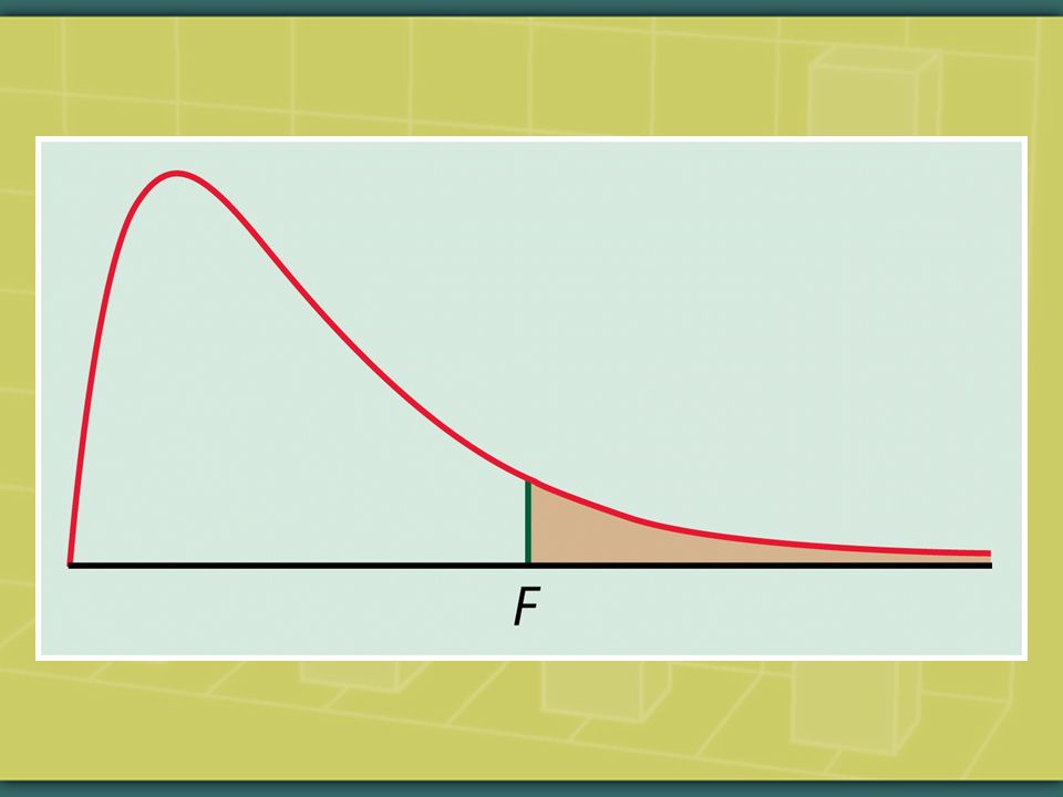
 Begin, then, with an F-test for overall model significance, before testing the slope coefficients. Ho: Ha: at least one F=Mean Square for Model/Mean Square for Error  The F-test examines if at least one of the regression coefficients has a statistically significant relationship with the outcome variable y.  Only if the F-test is significant do we then test for t-significance of the individual slope coefficients.

. reg math read write science  Interpretation?

. reg math read write science  F-statistic = 3229.08/39.69 = 81.36

 Like other tests of significance, F is the magnitude of the effect divided by the error term.

 To repeat, conduct the F-test for overall model significance, before testing the slope coefficients. Ho: Ha: at least one F=Mean Square for Model/Mean Square for Error  The F-test examines if at least one of the regression coefficients has a statistically significant relationship with the outcome variable y.  Only if the F-test is significant do we then test for t-significance of the individual slope coefficients.

t-tests of Slope Coefficients  Conduct a significance test (one or two- sided) for each slope coefficient. Ho: Ha: (or one-sided test: > or <)  Beware of Type I errors.

. reg math read write science  t-value for read =.306/.060 = 5.07

R 2  R 2 : the squared multiple correlation (capital R, vs. previous small-case r) measures the proportion of the outcome variable that is explained by the explanatory variables (i.e. degree of cluster around regression line).  R 2 is the square of the correlation of the predicted values of y with the observed values of y.  It tells us what percentage of y’s variance is accounted for by the model (i.e. the explanatory variables): higher R 2, greater fit.

. reg math read write science  R 2 : Model SS/Total SS=9687.25/17465.79 = 0.55

 R-squared, however, is much less preferred than the slope coefficients as an indicator of model fit.  Recall the difference between ‘historicist’ & ‘generalizing’ explanation.  Simply adding more explanatory variables—even if they’re meaningless— will increase R-squared.

How to do multiple regression in Stata?

 Example: How much do science achievement test scores depend on reading achievement test scores & math achievement test scores in a random sample of 200 high school students?

 If there are any missing observations:. mark complete. markout complete science read math  Alternatively: perhaps save a working data set that excludes the missing observations.

 Regarding mark & markout: ‘complete’ is an binary, or dummy, variable: 1=complete data 0=incomplete data. tab complete

. gr matrix science read math if complete==1, half

. kdensity science if complete==1, norm. gr box science if complete==1. kdensity read if complete==1, norm. gr box read if complete==1. kdensity math if complete==1, norm. gr box math if complete==1  ‘complete’ is a binary, or dummy variable: 1=complete data, 0=incomplete data

. su science read math if complete==1, detail

. pwcorr science read math if complete==1, obs sig bonf star(.05) sciencereadmath science1.0000 200 read0.6302*1.0000 0.0000200 math0.6307*0.6623*1.00000.0000 200200 200  Note this way of using pwcorr (‘if complete==1’) corresponds to how regression uses the observations.

Correlation ci’s. ci2 read write if complete==1, corr. ci2 read science if complete==1, corr. ci2 write science if complete==1, corr Confidence interval for Pearson's product-moment correlation of read and write, based on Fisher's transformation. Correlation = 0.597 on 200 observations (95% CI: 0.499 to 0.679) Confidence interval for Pearson's product-moment correlation of write and science, based on Fisher's transformation. Correlation = 0.570 on 200 observations (95% CI: 0.469 to 0.657) Confidence interval for Pearson's product-moment correlation of write and science, based on Fisher's transformation. Correlation = 0.570 on 200 observations (95% CI: 0.469 to 0.657)

 ‘Partial coefficients’—correlation coefficients of the outcome variable with the explanatory variables, for each variable holding the others constant—are also helpful:. pcorr science read math if complete==1 Partial correlation of science with Variable | Corr. Sig. -------------+------------------ read | 0.3654 0.000 math | 0.3668 0.000  Compare partial correlations to correlations.

 Here are the hypotheses that we’ll test.

.Ho: Ha: at least one check for F-test significance.Ho: Ha: check for t-test significance

. reg science read if complete==1 science | Coef. Std. Err. t P>|t| [95% Conf. Interval] -------------+--------------------------------------------------------------------- read |.6085207.0532864 11.42 0.000.503439.7136024 _cons | 20.06696 2.836003 7.08 0.000 14.47432 25.65961 ------------------------------------------------------------------------------------. reg science math if complete==1 science | Coef. Std. Err. t P>|t| [95% Conf. Interval] -------------+---------------------------------------------------------------------- math |.66658.0582822 11.44 0.000.5516466.7815135 _cons | 16.75789 3.116229 5.38 0.000 10.61264 22.90315

. reg science read math if complete==1 Source SSdf MS Number of obs= 200 F( 2, 197)= 90.27 Model 9328.73944 2 4664.36972Prob > F= 0.0000 Residual 10178.7606197 51.6688353R-squared= 0.4782 Adj R-squared= 0.4729 Total 19507.50199 98.0276382Root MSE= 7.1881 science Coef.Std. Err. tP>t[95% Conf.Interval] read.3654205.0663299 5.510.000.2346128.4962282 math.4017207.0725922 5.530.000.2585632.5448782 _cons 11.61553.054262 3.800.0005.59225517.63875  What might happen to the slope coefficients if we add other explanatory variables? Why?

 Here’s a quick, simple way to graph regression coefficient ci’s in multiple regression:. reg science read math if complete==1. gorciv read math

 See ‘Graphing confidence intervals in Stata’ for the commands ‘parmby,’ ‘sencode,’ & ‘ecplot’ to make more useful graphs.

. Check that N-observations is correct in the model.. predict yhat if e(sample). predict e if e(sample), resid. hist yhat, norm. hist e, norm. rvfplot, yline(0). sort science [to order low-high values]. list science yhat e. lvr2, ml(id). lincom _cons + read*45 + math*45. lincom _cons + read*65 + math*65

 The residuals are approximately normal in distribution.

 There might be some rightward tilt worth exploring. We can use ‘rvpplot’ to explore individual variables.

. rvpplot read, yline(0). rvpplot math, yline(0)  There might be some minor problem with read’s relationship with math.

 lvr2plot: let’s estimate the model with & without id=167 to see if there’s a notable difference.

 There’s some difference, but nothing that will change the interpretation of the results.. reg science read math if complete==1

 Results: the regression model provides a good fit: there are significant relationships between y & the explanatory variables, with meaningful magnitudes.  The residuals are more or less properly distributed; & the one influential outlier doesn’t make any major difference.

 Let’s try to improve the model by adding a new explanatory variable, ‘white,’ which is coded 0=nonwhite 1=white.  A binary categorical variable coded 0/1 is called an indicator, or dummy, variable.

. tab white. su science, d. ttest science, by(white) [exploratory hypothesis test]

. ttest science, by(white) Two-sample t test with equal variances Group Obs Mean Std. Err. Std. Dev.[95% Conf. Interval] nonwhite 55 45.65455 1.255887 9.31390543.13664 48.17245 white 145 54.2.7552879 9.0948752.70712 55.69288 combined 200 51.85.7000987 9.90089150.46944 53.23056 diff -8.545455 1.44982 -11.40452 -5.686385 Degrees of freedom: 198 Ho: mean(nonwhite) - mean(white) = diff = 0 Ha: diff 0 t = -5.8941 t = -5.8941 t = -5.8941 P t = 0.0000 P > t = 1.0000

. reg science read math white if complete==1 Source | SS df MS Number of obs = 200 ------------+------------------------------ F( 3, 196) = 70.84 Model | 10148.3965 3 3382.79884 Prob > F = 0.0000 Residual | 9359.10349 196 47.750528 R-squared = 0.5202 ------------+------------------------------ Adj R-squared = 0.5129 Total | 19507.50 199 98.0276382 Root MSE = 6.9102 ------------------------------------------------------------------------------ science | Coef. Std. Err. t P>|t| [95% Conf. Interval] ------------+---------------------------------------------------------------- read |.3227622.0645911 5.00 0.000.1953793.450145 math |.380627.0699709 5.44 0.000.2426345.5186194 white | 4.719807 1.139193 4.14 0.000 2.473158 6.966456 _cons | 11.53217 2.936238 3.93 0.000 5.741491 17.32284 ------------------------------------------------------------------------------  Interpretation?

 Interpretation of the dummy variable: the science scores of ‘whites’ are 4.7 points higher than those of ‘nonwhites,’ on average, other explanatory variables held constant.

. drop yhat e. Check that N-observations is correct in the model.. predict yhat if e(sample). predict e if e(sample), resid. hist yhat, norm. hist e, norm. sort science. l science yhat e. rvfplot, yline(0). lvr2plot, ml(id). lincom _cons + math*45 + white. lincom _cons + math*45 – white  Go through the model-assessment steps: Is this an improved model or not, & why?

 Our discussion of linear regression brings us back to an earlier topic: linear transformations (Moore & McCabe, pages 51-55).

 Recall that multiplying each observation by a positive number b multiples both measures of center & spread (i.e. variance & standard deviation), thereby increasing dispersion (i.e. inequality).  Recall also that adding or subtracting the same number a to observations adds a to measures of center & to quartiles & other percentiles but does not change measures of spread.

. gen xsci=5*science. univar science xsci Variable n Mean S.D. Min.25 Mdn.75 Max ------------------------------------------------------------------------------- science 200 51.85 9.90 26.00 44.00 53.00 58.00 74.00 xsci 200 259.25 49.50 130.00 220.00 265.00 290.00 370.00. gen asci=5 + science. univar science asci Variable n Mean S.D. Min.25 Mdn.75 Max ------------------------------------------------------------------------------- science 200 51.85 9.90 26.00 44.00 53.00 58.00 74.00 asci 200 56.85 9.90 31.00 49.00 58.00 63.00 79.00 -------------------------------------------------------------------------------

 Other kinds of transformations, however, are not linear but, rather, nonlinear (see McCabe & Moore, pages 187-203).  In contrast to linear transformations, nonlinear transformations potentially can normalize a variable’s distribution & straighten a curved relationship between two variables.

 Why might we need to straighten out a skewed univariate distribution or a curved relationship between two variables? (1) A skewed distribution may be difficult to examine became many observations may be piled up in one place or some observations may be hidden; & summary measures such as mean & standard deviation are distorted by skewed distributions.

(2) Linear relationships are easier to interpret; statistical theory is better developed for linear relationships; & nonparametric statistics are not as insightful as parametric statistics. (3) A curvilinear relationship causes invalid results for correlation and regression.

 The nonlinear transformations that we’ll briefly consider will consist of logarithms, powers & roots.  Remember: for correlation and regression, what really matters are not univariate distributions but rather bivariate relationships as displayed in scatterplots.  So, for correlation and regression, don’t make decisions about transformations until you’ve inspected the scatterplots.

 Keeping the preceding point in mind, Stata makes choosing among potential non-linear transformations relatively easy.  Using data on household consumption per capita in Tegucigalpa data:. kdensity dhc, norm. qladder dhc

. kdensity dhc, norm scheme(economist)

. qladder dhc

 qladder dhc suggests that a log transformation of dhc will make its distribution more normal.  gen ldhc = ln(dhc)  su dhc ldhc  for varlist ldhc-dhc: kdensity X, norm \ more

. kdensity dhc, norm

. kdensity ldhc, norm

 The log transformation did considerably normalize the variable’s distribution (by dampening the effect of the right-skewed distribution’s high-end values).

 The ‘qladder’ command is based on John Tukey’s ‘ladder of power transformations’ (see Moore & McCabe, pages 191-95; & see Stata’s command ‘ladder’).  See the ‘ladder’ command for a hypothesis- test based approach to selection.  The ladder of transformations recommends particular non-linear transformations for particular non-linear relationships.

 While the ‘ladder’ does help, normalizing a variable’s distribution & linearizing a bivariate relationship generally involve trial & error.  And not all skewed distributions or non-linear bivariate relationships can be straightened out in a satisfactory way.

 There’s always a trade-off, moreover: A nonlinear transformation may indeed normalize a variable or linearize a relationship between variables, but a significant cost may be diminished clarity of interpretation.  Remember: what really matters is the scatterplot, not the univariate frequency distributions.  So don’t make decisions about transformations until you’ve inspected the scatterplot.

 There’ll be lots more transforming next semester.

Interaction Effects  One more thing: what if the relationship of y to x varies according to the level of another variable, z?  This is an ‘interaction effect’.  E.g., do not drink alcoholic beverages while taking medication X.  E.g., the effect of an educational intervention varies according to the gender of students.

 A regression example: with regard to the log annual household living standard measurement per capita of a stratified random sample of households in several collective agricultural communities (‘ejidos’) in Quintana Roo, Mexico.  The value of the outcome variable increases with higher farm levels of mahogony production & with presence (vs. absence) of a community saw mill.  Is there an interaction effect between mahogony production level & mill presence/absence?

. twoway scatter lsm mvc || lfit lsm mvc, by(mill)

 Interaction: coef=1.24, p=.000

 postgr3 mv, by(mill) table: graph of saw mill X mahagony volume categories (see next slide)

. postgr3 mvc, by(mill) table [predicted average values of lsm by millXmvc] Variables left asis: mvc _Imill_1 _Imi1Xmv Holding hway constant at.79396985 Holding nmaya constant at.46231156 Holding resworks constant at.71356784 ------------------------------ Mahogany | volume | categorie | Mill s | No mill Mill ----------+------------------- 0 | 3.738333 1 | 3.718388 2 | 3.446435 3 | 3.678499 4 | 5.879803 ------------------------------

. findit xi3 [download]. help xi3. findit postgr3 [download]. help postgr3. xi3: reg y x i.xcat*z. postgr3 x, by(xcat)

. twoway scatter yhat mvc if mill==0 || mspline yhat mvc if mill==0, clpatt(solid) || scatter yhat mvc if mill==1, ms(oh) || mspline yhat mvc if mill==1, clpatt(solid) ||, ytitle("Ave. Living Standard Measure")  Another way to graph the interaction

 As an alternative to postgr3, table or to complement interaction graphs in general, use lincom to explore predicted outcomes.  See Paul Allison, Multiple Regression: A Primer.  See the next slide…. reg lsm hway mvc mill mvcXmill nmaya resworks

 You’ll spend lots of time analyzing interaction effects next semester.

 On making correlation & regression tables, see the class document ‘Making working & publication-style tables in Stata’.

. findit esttab [download]. findit eststo [download]. reg lsm hway mill mvc nmaya resworks. eststo. reg lsm hway mill mvc millXmvc nmaya resworks. estso. esttab, se starlevels(+.10 *.05 **.01 ***.001) r2 nodepvars no mtitles compress

Review: Correlation vs. Regression  What are the main differences between correlation & regression?  What are the data requirements for each?  What.

Similar presentations

Presentation on theme: "Review: Correlation vs. Regression  What are the main differences between correlation & regression?  What are the data requirements for each?  What."— Presentation transcript:

Similar presentations

About project

Feedback

Log in

Auth with social network:

Review: Correlation vs. Regression  What are the main differences between correlation & regression?  What are the data requirements for each?  What.

Similar presentations

Presentation on theme: "Review: Correlation vs. Regression  What are the main differences between correlation & regression?  What are the data requirements for each?  What."— Presentation transcript:

Similar presentations

About project

Feedback