2. The following presentation shows most of the features available in the Emax Analyzer Program written by Mike Glazer. This program allows analysis of log file data downloaded from Avidyne and Arnav multifunction displays (MFD), as fitted to Cirrus and Lancair Columbia aircraft. Click for next slide

3. This is the opening screen Start by clicking on File Let’s begin by showing standard one-off reading of an Avidyne log file.

4. Click on Open Or else if you have previously loaded log files you can choose here You may need to select Avidyne or Arnav first to read in correct log file Don’t worry about him!

5. Navigate to the folder on your computer where you have stored all the log files downloaded from your MFD. Highlight a log file (ignore small files of about 7kB or less as these are probably junk files created whenever you just switch on the engine.

6. The first chart that opens is your EGT’s

7. Pointing with the mouse to any position on a trace highlights that trace and shows the values at that point

8. Pointing with the mouse to an entry in the legend also highlights that trace

9. Pointing and dragging with the left mouse button to expand any area

10. With the right mouse button you can move the plots around

11. Click on button to return to original size

12. or with the left mouse button drag from lower right to upper left and release to return to original size

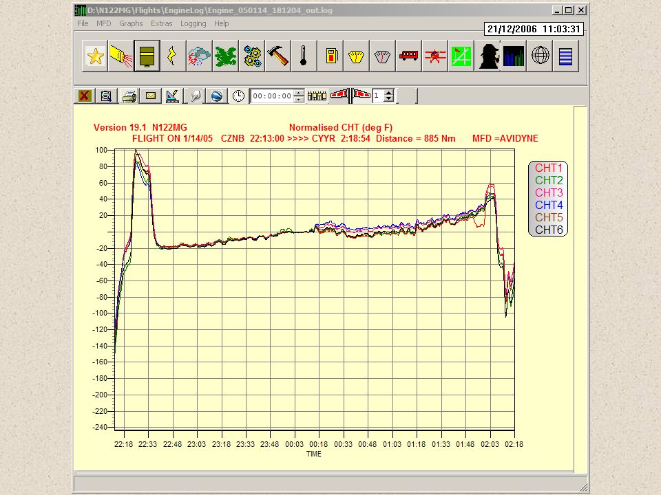
13. Here is the CHT plot Note that by pointing to a particular place on a CHT or EGT curve and clicking you can renormalise all the traces to this point

15. This shows how the CHT’s change with time (derivative curves). Any CHT that misbehaves should be seen as a blip on any curve

16. Clicking on the altitude button will plot altitudes, provided your aircraft is provided with a sensor to report this. Mine doesn’t!! By the way, note that at the bottom a time increment is shown. Just dial up how much time you wish to add to the time axis and click here to activate. The time axis should now be increased

17. This shows the oil temperatures and pressures

18. This shows the RPM and MAP

19. ROP (Rich of Peak) power and LOP (Lean of Peak) power are shown here. Choose your aircraft here, Cirrus SR20, SR22 and three types of Lancair Columbia

20. Outside air temperatures in degrees Celsius and Fahrenheit Note that on any screen double clicking with the left mouse button opens up the relevant Help screen

21. Fuel flow and amount of fuel used during the route Note information written at top

22. From the Extras menu item choose “Add Comment” to add your own information

23. Comment added

24. Bus voltages

25. Successive clicks on the Smoothing button makes the curves smoother

26. Plot of mean ground speed, actual ground speed at any time, and nautical miles per gallon. This plot really could do with smoothing.

27. That’s better!

28. Go to menu item Extras and click on “Mark Line”

29. A yellow vertical line that you can drag to any position. Useful if you want to indicate a particular event and send the image to someone for comment

30. Click here and nearest airfields and beacons are indicated at the correct places. Subsequent clicking increases the range for finding airfields and beacons. After several clicks, this returns to the shortest range.

31. Go to menu item Extras and choose “Combinations”.

32. Here I have selected all EGT’s and CHT’s with scale on left axis plus Fuel Flow on right axis. Click here if you want to save combination

33. If you have clicked on Custom Chart then this particular combination will be saved and shown at any time by clicking on My Custom Chart Button.

34. Now let’s look at some other buttons

35. The first button is a Print Preview and the second is to send the diagram to the printer

36. Send the chart by email

37. This button allows you to change the Chart settings e.g. change color of plots etc.

38. From the File menu item choose “Save Settings” if you wish to save the Chart settings. “Default Settings” returns to the original settings and “Read Settings” reads your saved settings.

39. From the File menu item choose “Change File Names”. This was put in there for our leader Mike Radomsky. What it does is to add your tail number to the front of each log file name so that you can immediately identify which aircraft the log files belong to. It only works on individual log files.

40. This sends your route data to Google Earth (you have to have this already installed on your computer first).

41. You can choose line widths and color for your route plot in Google Earth. The Range of Air Data determines how far from the route airfields and beacons should be marked. If altitude data are available then check the “Use Altitude Data” box.

43. Click to show EGT and CHT variations from average temperatures in your engine. Note how in my engine at this time the CHT is 7% higher than the average (probably means a cooling problem). Click again to cancel.

44. How to measure the GAMI spread The idea here is to find out as you slowly lean your mixture the difference in fuel flow from when the first cylinder peaks to the last. The smaller the GAMI spread (typically less than about 0.5 gals/hour) the better balanced you cylinders are. In order to run LOP successfully you need to have a small GAMI spread. So this is what you do. Fly your aircraft in the cruise say at about 8000 feet. Then slowly lean the mixture until you have passed through the peak EGT’s on all cylinders. After downloading your log file, use the Sherlock Holmes button.

45. Find the region where the GAMI spread measurement is to be taken. Make sure the peaks are more or less in the center of the graph with the ‘tail’ on the right hand side. peak tail

46. Now click on the Sherlock Holmes button. Nice GAMI spread!!! It is rarely that good. Click again on Sherlock Holmes to close GAMI spread box

47. Let’s simulate the MFD during this flight. Click on Simulation box.

48. Pause Run Speed After pause slide to event Make EGT’s absolute Normalise the EGT’s Celsius or Fahrenheit Stop simulation

49. Pull down with left mouse button to resize Click on a chart button to see progress. Note yellow marker moves in sympathy with simulaton Right click closes simulation

50. In Version 20.3 I have added some more functionality to the simulation page

51. Single step, holding key down repeats continuously Trend indicators

52. This is an example where I have used the single stepping to show a mag fault during a LOP mag check. Cylinders 1 3 and 5 decrease in temperature rather than rise. Readjusting the mag solved the problem in this case.

53. Go to Extras and Listing to obtain a full listing of the Log File.

54. Go to Extras and Tail Number to change Aircraft sign

55. Click here to plot route

56. Click for default scale

57. Click for World scale

58. Choose high-resolution coastline mapping.

59. Click for direction arrows

60. Notice latitude and longitude data given as the mouse cursor moves across the screen.

61. Pointing to a place on the actual route gives the time, track and ground speed. Notice how fast it was because of strong winds! Note CHT information on bottom status bar.

62. How about this? During the subsequent ferry flight from Iceland to Holland my aircraft achieved a ground speed of 251 kts!!! Incidentally, a red line indicates that during this part of the route a CHT exceeded 390F

63. Click to enlarge or reduce. Can also be enlarged by dragging with the mouse and left mouse button

64. Click to draw airfield and name. Second click marks with ICAO or airfield code

65. Click to mark beacons

66. Click here to watch the route progress. Speed is controlled by slider below.

67. Click for return to fast route plot

68. Controls for moving image left, right, up and down

69. Clicking on any of these buttons returns you to charts

70. And now how to log all your flights

71. Click on this button or go to the menu item Logging/Show Logs to open up the Flight Log page.

72. This is a blank Flight Log page. Click on the + button to add flights.

73. Enter the registration number (tail number) and press OK

74. Navigate to the folder where you keep your log files. You may find so-called track files in this folder. The Emax program will automatically avoid reading these in, but for safety it is best to remove them first.

75. Click on the Size label twice to place all the files into descending order of size. You can now highlight all the files from the biggest to the smallest (don’t bother with files smaller than about 8kB), and press Open.

76. Chances are you will get a message like this. It means that these log files are probably faulty. Click on the blank line below the stars to continue or on one of the faulty file names to view.

77. So here is our summary flight log. By clicking on the titles of each column you can often order the entries.

78. Scrolling to the right shows more information for each entry, in particular the location of the relevant file. Please note that if you move the log files to another folder the program cannot find them. You can find a.sum file in your folder and edit this to substitute the new folder locations.

79. If you highlight an entry, and then right click on that entry (or click on the graph button) you will be taken immediately to the charts for that file.

80. Clicking on the pennants enables you to load each log file sequentially in order to watch changes from log file to log file.

81. Clicking on the number in this box causes all the log files to be shown in a timed sequence. Changing the number changes the speed. This works on any of the charts.

82. Clicking on the aircraft button opens a list box showing the different aircraft logs. So you see you can actually store several different aircraft logs. Highlight the one you want and double click.

83. Highlight a line and then use this button to remove the entry.

84. With this button you can erase the whole flight log.

85. With this button you can print the flight log.

86. Click on this to see certain trends.

87. Maximum values of EGT, CHT, Oil pressure and Oil temperature are plotted against flight number. Point to any flight on a curve and click: the charts for that flight will be opened up.

88. Notice that you can email this plot.

89. This what you get with smoothing.

90. Click on this to change the limits used in plotting the trend graph. Useful if you want to remove say meaningless spikes.

91. I think this should be fairly obvious how this works

92. Now let’s try this button.

93. So this shows how the CHT’s change from the average values with flight number. Notice near flight 41 (see vertical line) CHT2 and CHT6 changed as a result of changes to the baffling at an annual service. The plot has been smoothed here

94. Click here to see the trends for EGT’s

95. The odd behavior for EGT5 is due to a probe fault. Note that when this indicates low it causes the other average values to seem to increase.

96. In Version 19.3 there are two new buttons Press the left one to change flight times to estimated Hobbs times (assumes timing whenever ground speed exceeds 40 knots) Press the right one to return to ordinary flight times

97. In Version 19.3 there yet another new button This allows you to export the Flight Log to a.CSV file suitable for importing into Microsoft Excel.

98. So you have now seen most of the important functions. The following shows an example of how the program can diagnose a particular engine fault This aircraft, an SR20, suffered a catastrophic failure of cylinder 4.

99. This is the CHT behavior on the penultimate flight. Notice how CHT4 is always much lower than the others. Earlier flights did not show this as much. This is consistent with a blocked injector on cylinder 4.

100. The same flight with the fuel flow and EGT’s added. Note that the fuel flow shows this aircraft to be just LOP during the cruise phase. Being LOP, the blocked injector would make CHT4 decrease as is seen.

102. Sudden rise of EGT4 Rise of CHT4 above 500F: Note values above 500F are assigned 0 value by Avidyne Catastrophic failure of cylinder 4 Fuel flow indicates ROP

103. Lesson A blocked fuel injector when flying ROP can lead that cylinder to get hotter and cause detonation followed by preignition, as happened here. Flying LOP with a blocked injector,as in the penultimate flight, only caused harmless cooling of that cylinder. Had the pilot noticed the rapid CHT rise he could have taken action to avoid the preignition event by using full mixture and low power.

104. Looking back on all the flights we can even trace approximately when the injector for cylinder 4 started to block. Roughly from the arrow onwards we see that CHT4 progressively decreases with respect to the other CHT’s.

105. The rise of CHT4 here can be traced to running just ROP.

106. Note that most of the time the aircraft is being flown ROP, above the green line.