1. EC 2333: Topic 6: Slavery and its Aftermath Professor Robert A. Margo Spring 2014

2. Outline Background on economics of US slavery: Fogel and Engerman (1974, etc.) + Fogel (1989) Central topic in 1970s-80s; quieted down in 1990s, 2000s BUT has picked up again sharply. Today: Basics of Fogel +Engerman and Post-bellum South. Class presentation on Naidu; Boustan. Other recent work of importance: Miller; Chay-Munshi; Olmstead-Rhode; Collins and Wanamaker Separate subject: evolution of Black/White income differences in C20 (Boustan is part of this literature).

3. Key Features of Slavery Slavery is VERY common throughout human history, found in many societies throughout the world (relationship to war) Essence of slavery → Owner has “control” over the slave’s human capital Status is involuntary, typically is also inherited Owner can buy and sell: market for slaves Span of control varies enormously across societies and over time

4. Why Slavery? Domar model: when labor/land ratio is very low and MP(labor) is very high, owners of land have an incentive to limit labor mobility Example: feudalism North and Thomas: population growth → diminishing returns → pressure to establish new manors→ incentives → labor becomes more “free”

5. Why Study Economics of US Slavery? Slavery and Regional Development Within US: North “Industrializes”, South does not South as “Economic Problem”: Early 20 th Century Role of Slavery in Coming of Civil War Racial Economic Differences in 20 th Century US: Role of Slavery

6. Context: Slavery and Southern Development Old View: Slavery made the southern economy “moribund” Evidence? South seemed very poor in early 20 th century, economically “backward” Why? Slavery was an “archaic”, “pre- capitalistic” economic system

7. New View: Easterlin Estimates Richard Easterlin (1961): Regional Estimates of Per Capita Income, 1840-1950 by 20-year time periods (eg. 1840, 1860, etc.) Pre-Civil War per capita in South is below national average BUT Income per White Southerner > National Average Growth Rate of Per Capita Income in South Before Civil War at About National Average Dramatic Decline in Southern Per Capita Income Relative to National Average Between 1860 and 1880 Problems with Easterlin (1) No Adjustment for Regional Differences in Cost of Living (2) Output in North Central May be Biased Downward

8. Easterlin Estimates, 1840-80: Relative Per Capita Income 184018601880 National Average 100 Northeast135139141 North Central 68 98 South 76 72 51

9. Profitability of Slavery Profitability of Slavery: Very Old Issue Plantation Studies: Phillips, Sydnor Conrad and Meyer: Internal Rate of Return→ value of r that equates asset price with present discounted value of expected net product (net product = gross product – maintenance) Conclusion: return on slavery > next best alternative (adjustment for risk?) except in S. Atlantic → westward migration Fogel and Engerman: large sample of slave sales + rental contracts (NOTE: much more is available today) Conclusion: slavery was profitable

10. Viability of Slavery However, profitability ≠ viability (Yasuba 1961) Viability: does it “pay” for slave system to “reproduce” itself? Related to economics of “manumission”: relatively uncommon in ante-bellum South Fogel and Engerman: price of new-born slaves (3 percent of price of prime-age male) > 0: capitalized rent True in 1860: No evidence slavery was about to die out on eve of Civil War Problem: price of new-born slaves is estimated, not observed

11. Why Was Slavery Profitable and Viable? Slaves were “Exploited” Economics of Exploitation: VMP > “W” (monopsony rents) Fogel and Engerman Estimate of W/VMP = 0.93 (slaves received 93 percent of value of marginal product): Disputed Slaves were exploited but may not be sufficient to explain profitability + viability

12. Relative Productivity of Slave Agriculture Fogel and Engerman resolution: slave agriculture was relatively productive “Relative”: compared to free agriculture in South and in the North NOT true in general but true in certain staple crops (cotton, tobacco, rice, sugar) Primarily due to use of “gang system”

13. Analysis of Productivity Based on “Parker-Gallman” Sample of Farms from 1860 Manuscript Census of Agriculture “Manuscript Census”: original hand-written census returns 19 th Century Surviving Manuscript Economic Censuses: Agriculture (1850-1880), Manufacturing (1820, 1832, 1850-1880) Available Samples, Agriculture: Parker-Gallman (1860 South), Bateman-Foust (1860 North), Ransom-Sutch (1880 South) Available Samples, Manufacturing: Atack-Bateman (1850-80 National) Parker-Gallman: sample from agricultural census matched to population census + slave schedules Source: ICPSR (University of Michigan, www.icpsr.umich.edu)

14. Approach Cobb-Douglas Production Function Ln V = ln A + α L ln L + α K ln K + α T ln T In some specifications, Σα=1 (constant returns to scale) Ln V = log value of output, evaluated at national prices Extensive modifications to L K is value of farm capital, T is value of farm land Initial findings (a) no evidence that A differed between free farms in North and South (b) slave farms had higher average value of A (c) slave productivity effect appears at approximately 15+ slaves Subsequent econometric refinements (Field, Loman)

16. Possible Explanations Fogel and Engerman: Gang System Gang system: division of labor in planting, cultivation, extensive monitoring Some similarities with factory system in manufacturing (which also had higher productivity) Free labor unwilling to work in a gang except at a wage that would have made the gang system unprofitable Slavery enabled slave owners to reap the profits of gang labor Because agriculture was a competitive industry, cost advantages were passed onto consumers and output and resources shifted towards the gang system over time Explanation disputed by Olmstead and Rhode. Plantations were not “factories in the field”. Other explanations: omitted variable bias, systematic errors in outputs or inputs correlated with use of slave labor, endogeneity of crop mix, year effect (1860)

17. The Aftermath of Slavery Aftermath of Slavery: “Post-bellum South” Why Important? (a) ca. 1900 the South appears to be very poor, does not really “converge” on rest of the economy until much later in 20 th century (b) 90 percent of African-Americans live in the South ca. 1900 (c) institutionalized racism (“Jim Crow”, disenfranchisement, de jure segregation)

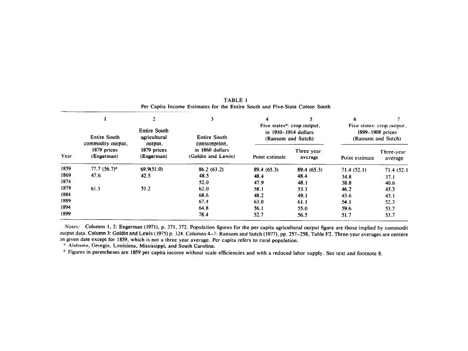
18. Decline in Southern Income Engerman (1971) estimated regional distribution of per capita “commodity” output South/Non-South per capita income declines sharply between 1860 and 1880 (approximately a third) More detail in Ransom and Sutch (1977) and Goldin (EEH, 1979)

20. Why the Initial Decline? Ransom and Sutch: reduction in labor force participation in the South Temin (also Wright): decline in demand for Southern cotton F&E: loss of economies of scale due to emancipation Goldin (1979, EEH): ½ due to loss of economies of scale, 1/3 to decline in L/P, 1/6 to decline in demand for cotton Good idea to redo Goldin using more recent work on economies of scale and, especially, labor force participation (Weiss) Irwin (EEH, 1994): uses county level data in regression context; loss of economies of scale is the dominant factor

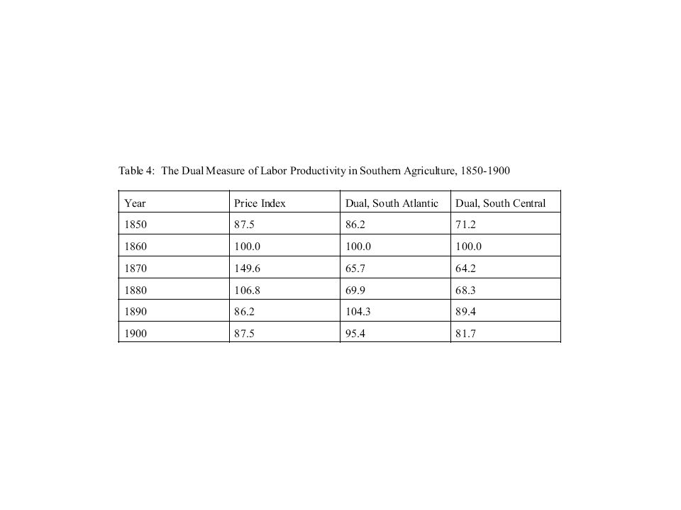
21. Margo (2004) Previous evidence on regional wage divergence (Wright) very limited Sources are published and archival Estimates of “real product wage” (dual = productivity measure) in southern agriculture Dual (w/p) suggests decline in labor productivity New evidence on cost of board

22. Key empirical findings S/N wage ratios decline sharply after the Civil War; decline is immediate Decline is widespread across occupations, larger in magnitude in Deep South Short run decline > Long run decline By 1890, wage ratios about at antebellum level for non- farm labor Only small portion of decline can be attributed to changing racial composition of postbellum wage labor force in South Time series of w/p (dual) suggests two shocks, 1860s and 1890s, 1860 is “once and for all” Decline in S/N relative price of non-traded goods

23. “Theory” In an economy with “localized” factor markets, “shocks” will have short run effect Negative shock to labor demand: wages and non-traded goods prices fall (contrast with negative shock to labor supply) Simple model: (1) south produces “cotton” and X (non- traded good) (2) southerners consume X + traded good (“manufactures”) (3) price of C and M set on world market (4) aggregate regional factor supplies are fixed (5) C produced initially with slave labor but X is produced using free or slave (perfect substitutes) Shock: gang system no longer feasible Predictions: Short run, w falls, p(x) falls; long run, eventually labor migrates

24. Evidence Published evidence: USDA (daily and monthly wages of farm labor, with and without board; daily wages of skilled artisans, 1880, by occupation); weekly wages of female domestics, 1870 and 1900, 1890, 1900 common labor, from Lebergott (1966) Unpublished evidence: 1850-70 Census of Social Statistics, 1880 manuscript census of manufactures, Reports of Persons and Articles Hired (civilian workers at military installations)

25. Tables 1 and 2 Table 1 shows S/N wage ratios for farm labor, common labor, carpenters, and domestics Sharp decline in short run Some recovery by 1880s but appears to be a second shock in 1890s Table 2: decline is larger in the Deep South Not shown: decline occurs within stages (Virginia versus West Virginia)

29. Table 3 A possible explanation involving race AA share of wage labor MUCH larger after Civil War than before If AA receive lower wages because of discrimination, this may explain decline (NOTE: what about recovery?) Evidence is meager but suggests that racial wage gaps for common/farm labor were small

31. Table 4 Under competitive assumptions, W/P measures labor productivity (“dual”) where P = price of output Price index for southern agriculture constructed from Towne and Rasmussen W/P declines sharply from 1860-1870, recovery in 1880s, further decline in 1890s Measuring effect of emancipation is difficult because we have only two data points before Civil War

33. What About Other Factor Prices and Factor Quantities? Increase in interest rates/cost of capital: financial disruption, destruction of capital stock w/r falls → K/L should decrease, which reduces labor productivity Strong evidence of decrease in K/L in manufacturing (Hutchinson and Margo 2005)

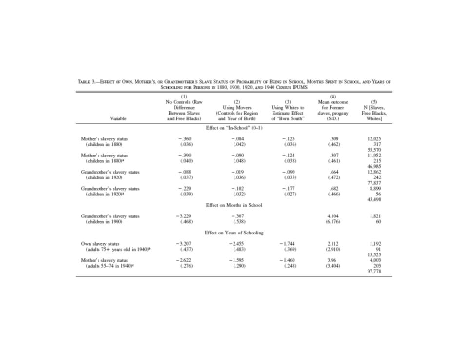
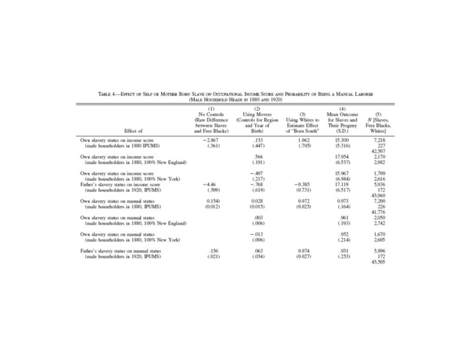
37. Sacerdote (2005, RESTAT) Most studies focus on AA/W convergence However, recall previous slide on illiteracy: within race, convergence in illiteracy between southern and non-southern born AA Sacerdote is different: comparison between children of free blacks vs. former slaves Since (vast) majority of free blacks were descendants of former slaves, comparison is really between recent and distantly freed slaves Idea is to distinguish impact of slavery per se Bottom line: at end of Civil War, significant gap in (literacy, school attendance, occ status) between free blacks and former slaves BUT gap is closed (more or less) in approximately two generations (i.e. by 1920) Consistent with “intergeneration transmission coefficient” of 0.3-0.5: modern studies

38. Sacerdote: Analysis Three estimators Sample #1: Free blacks + former slaves, compare outcomes Estimate #2: #1 + controls for current region, identifies slavery effect from movers Estimate #3: uses whites as “control group” #3 (and #1) overstate effect, #2 understates Sacerdote: “true” effect is between #2 and #3

39. Sacerdote: Findings Estimate #1: large in 1880, much smaller in 1920 Estimate #2< Estimate #1 Estimate #3> Estimate #2 Substantial convergence between slaves and free blacks by 1920 Interpretation: (1) negative effect of slavery per se WITHIN race diminishes substantially within two generations (2) Race (and current discrimination) VERY important in early 20 th century, society does NOT distinguish within race based on former slave status