1. Optimal Groundwater Remediation Laura Place Taren Blue

2. Outline Background – What is Groundwater Remediation – Major Contaminants and Contamination Areas The Remediation Process – Treatment Methods – Mathematical Models Optimization Completed Work Fluid Flow Modeling Plans and Recommendations for Future Work

3. Background Groundwater Remediation – Removal of contaminants from a water supply Standards set by the EPA – Several methods for treatment Existing Experimental – Optimization Mathematical models

4. Background Sources of contamination – Industrial & agricultural Storage tanks Septic systems Landfills Hazardous waste sites Road salts Refinery operations Mining Other chemicals

5. Contaminants, Possible Health Affects, EPA Standards CompoundPotential Health AffectsSources of Contamination BenzeneKnown Carcinogen Discharge from factories, leaching from gas storage tanks and landfills †,†† Vinyl ChlorideKnown Carcinogen Leaching from PVC pipes, discharge from plastic factories †,†† Arsenic Skin damage or problems with circulatory systems, and may have increased risk of getting cancer Erosion of natural deposits, runoff from orchards, runoff from glass & electronicsproduction wastes †† Copper Gastrointestinal distress, liver or kidney damage, and more Corrosion of pipes and household plumbing systems, erosion of natural deposits †† Lead Delays in physical and mental development in children, possible deficits in attention span and learning disabilities. Adults can experience kidney problems or high blood pressure Corrosion of pipes and household plumbing systems, erosion of natural deposits †† MercuryKidney damage Erosion of natural deposits, discharge from refineries and factories, runoff from landfills and crop lands. †† Trihalomethanes Liver, kidney or central nervous system problems, increased risk of cancerBiproduct of drinking water disinfection ††, ††† Nitrate In infants, could cause illness or death; characterized by shortness of breath or blue-baby syndrome. Runoff from fertilizer, leaching from septic tanks, sewage, and erosion of natural deposits. †† † Environmental Protection Agency Waterscience †† Environmental Protection Agency Safewater ††† National Water-Quality Assessment Program

6. Where are the Problem Areas? Arsenic Nitrates Hard Water VOCs

7. Optimization Goals – Minimize the remaining contaminants – Minimize cost Costs minimized are unique to the model – Other goals are also unique to the specific model – Optimizing the pump treat inject method (PTI) Number of wells Well configuration

8. Similarities & Differences of Previous Models

9. What are the Choices? “Dilution is not the solution!!!” – Inexpensive but never resolves the problem Pump, Treat, Inject method (PTI) – Pump contaminated water from the source (the plume) – Treat the water – Inject treated water back into the aquifer

10. PTI – Simple Schematic

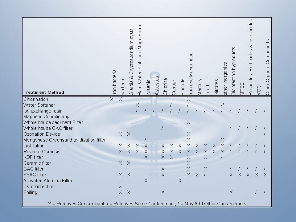
11. Treatments Existing treatment methods – Ion exchange chromatography – Membranes – “Point of service” treatment – Bioreactors – Adsorption – In situ bioremediation – Liquid-liquid extraction Surfactants

13. Challenges of Remediation Plume – Unknown flow patterns – Unknown concentration profiles Nonuniformities in concentration – Unknown position – Uncertainty in composition – Unknown size – Geological uncertainty

14. Problems and Affect on Treatment ***Modeling of the aquifer depends on many of these parameters. Therefore, all of these issues also become a problem in mathematical modeling.

15. PTI Has many parameters – Number and location of wells Few large wells Many small wells – Pumping Rate – Concentration of contaminants in treated water – Can vary well arrangement with time For optimization – Need a model!

16. Well Position and Treatment Four different well arrangements. ***Concentration profile of the plume is affected by location of pumping and injection wells.

17. Steps Completed in Optimization Analytical Model Euler Approximation – Optimization for minimum cost Initial Fluid Flow Modeling and Analysis Refined Fluid Flow Modeling and Analysis – Optimization for minimum contamination

18. Analytical Model

19. Set Up Euler Approximation Where dc/dt is the change in concentration with time F p is the pumping rate c in is the concentration into the slice c out is the concentration out of the slice V slice is the volume of the slice

20. Euler Method Model Calculates total remediation time Uses inputs for: – Volume of the plume – Time steps – Flow rate – Initial concentration – Desired end concentration Calculation in each cell loops until the change in outlet concentration is < 0.0001

21. Euler Results t1t1 t2t2

22. Cost Optimization

23. Fluid Flow Analysis Arrangement Example of one arrangement – multiple outlets with one inlet

24. Fluent Calculate mass flow rates in the plume – More accurate approximations of concentration profiles Characterize fluid flow in the aquifer – Vary well arrangement – Vary number of injection and extraction sites – Vary pumping rate

25. Geometry - Gambit 1 st “draw” geometry in Gambit Create injection and extraction locations which may be turned on or off. – For off – face is treated as a wall – For on – face is designated either mass inlet or outflow – Each face is labeled by location

26. Generic Geometry 20 10 A BC D E F G 1 2 3 4 5 6 7

27. Define Geometry in Fluent One inlet One outlet

28. Imaginary Planes Fluent analyzes flow patterns through planes ABC DE FGH IJK LMN OPQ

29. Example of Fluid Flow Field in Fluent Flow rate of 50 kg/s

30. Example of Fluid Flow Field in Fluent Flow rate of 5 kg/s

31. Example of Velocity Contours Flow rate of 5 kg/s

32. Excel Results from Fluent imported into Excel

33. Mass Balance C -18 C -14 C -10 Negative flux or positive flux dictates which concentration to use in the mass balance

34. Remediation Time and Flow Rate (4,4) (4,1) (2,2) (2,1) (1,2) (1,1) (1,4)

35. Conclusions of this Model Imaginary planes give an accurate estimate of flow through the aquifer Flux through the planes can be used to describe concentration profiles with time This model allows for understanding of general flow patterns with configuration Gives basis of comparison for future modeling techniques

36. New Modeling Strategy Pipes in the top of the aquifer – More realistic injection modeling – Flow characteristics re-evaluated Several plume types evaluated – Non-uniform initial concentrations – Different shapes Injection and extraction varied with time More realistic aquifer shape

37. New Geometry for Wells

38. Naming the Wells A B C D 1234567

39. Naming Imaginary Planes

40. Planes Through the x-direction -18 -14 -10 18 …

41. Horizontal Planes Horizontal planes also named individually for x, y and z location in the aquifer.

42. Configurations and Flow Profiles

47. Model Aquifer with Non-Uniform Concentration 3 plumes analyzed

48. Schemes for Treatment Plume 1 Step 1Step 2Step 3

49. Schemes for Treatment Plume 2 Step 1Step 2Step 3

50. Schemes for Treatment Plume 3 Step 1Step 2Step 3

51. Plume 1, Step 1

52. Plume 1, Step 2

53. Plume 1, Step 3

54. Plume 2, Step 1

55. Plume 2, Step 2

56. Plume 2, Step 3

57. Plume 3, Step 1

58. Plume 3, Step 2

59. Plume 3, Step 3

60. 3D Velocity Contours

61. Changing Configuration with Time Plume 1

62. Visualization of Concentration Plume 1 t = 4 dayst = 20 dayst = 50 dayst = 0

63. Changing Configuration with Time Plume 2

64. Visualization of Concentration Plume 2 Groundwater Remediation * University of Oklahoma – Chemical Engineering Taren Blue, Laura Place, ** Miguel Bagajewicz * This work was done as part of the capstone Chemical Engineering class at the University of Oklahoma ** Capstone Undergraduate students ** Capstone Undergraduate students t = 4 dayst = 20 dayst = 50 days t = 4 dayst = 20 dayst = 50 dayst = 0

65. Changing Configuration with Time Plume 3

66. Visualization of Concentration Plume 3 t = 4 dayst = 20 dayst = 50 dayst = 0

67. Conclusions Dynamic optimization - Changing well configuration with time – Allows for fairly good cleaning of contaminants – Can give more efficient – Can create step changes in concentration profile – Reaches a plateau in the cleaning process Different plume profiles can be modeled with this technique – Plume profile has a large effect on cleaning – Varying shape – Varying initial concentration profile – Efficiency of cleaning and configuration is highly dependent upon initial concentration profile

68. Future Work Better analyze non-x-directional flow Examine more economics Examine different pumping rates Vary time of well configuration change Analyze more plume profiles – Shape – Concentration Produce more accurate results for profile near injection and extraction

69. Questions Thank you!

70. Acknowledgements Miguel Bagajewicz Linden Heflin Jeffrey Harwell Benjamin Shiau Peter Lohateeraparp Rufei Lu Roman Voronov