Download presentation
Presentation is loading. Please wait.

1
MS&E 211 Quadratic Programming Ashish Goel

2
A simple quadratic program Minimize (x 1 ) 2 Subject to: -x 1 + x 2 ≥ 3 -x 1 – x 2 ≥ -2
 2 Subject to: -x 1 + x 2 ≥ 3 -x 1 – x 2 ≥ -2")
3
A simple quadratic program Minimize (x 1 ) 2 Subject to: -x 1 + x 2 ≥ 3 -x 1 – x 2 ≥ -2 MOST OPTIMIZATION SOFTWARE HAS A QUADRATIC OR CONVEX OR NON-LINEAR SOLVER THAT CAN BE USED TO SOLVE MATHEMATICAL PROGRAMS WITH LINEAR CONSTRAINTS AND A MIN-QUADRATIC OBJECTIVE FUNCTION EASY IN PRACTICE
 2 Subject to: -x 1 + x 2 ≥ 3 -x 1 – x 2 ≥ -2 MOST OPTIMIZATION SOFTWARE HAS A QUADRATIC OR CONVEX OR NON-LINEAR SOLVER THAT CAN BE USED TO SOLVE MATHEMATICAL PROGRAMS WITH LINEAR CONSTRAINTS AND A MIN-QUADRATIC OBJECTIVE FUNCTION EASY IN PRACTICE")
4
A simple quadratic program Minimize (x 1 ) 2 Subject to: -x 1 + x 2 ≥ 3 -x 1 – x 2 ≥ -2 MOST OPTIMIZATION SOFTWARE HAS A QUADRATIC OR CONVEX OR NON-LINEAR SOLVER THAT CAN BE USED TO SOLVE MATHEMATICAL PROGRAMS WITH LINEAR CONSTRAINTS AND A MIN-QUADRATIC OBJECTIVE FUNCTION EASY IN PRACTICE QUADRATIC PROGRAM
 2 Subject to: -x 1 + x 2 ≥ 3 -x 1 – x 2 ≥ -2 MOST OPTIMIZATION SOFTWARE HAS A QUADRATIC OR CONVEX OR NON-LINEAR SOLVER THAT CAN BE USED TO SOLVE MATHEMATICAL PROGRAMS WITH LINEAR CONSTRAINTS AND A MIN-QUADRATIC OBJECTIVE FUNCTION EASY IN PRACTICE QUADRATIC PROGRAM")
5
Next Steps Why are Quadratic programs (QPs) easy? Formal Definition of QPs Examples of QPs
 easy Formal Definition of QPs Examples of QPs")
6
Next Steps Why are Quadratic programs (QPs) easy? – Intuition; not formal proof Formal Definition of QPs Examples of QPs – Regression and Portfolio Optimization

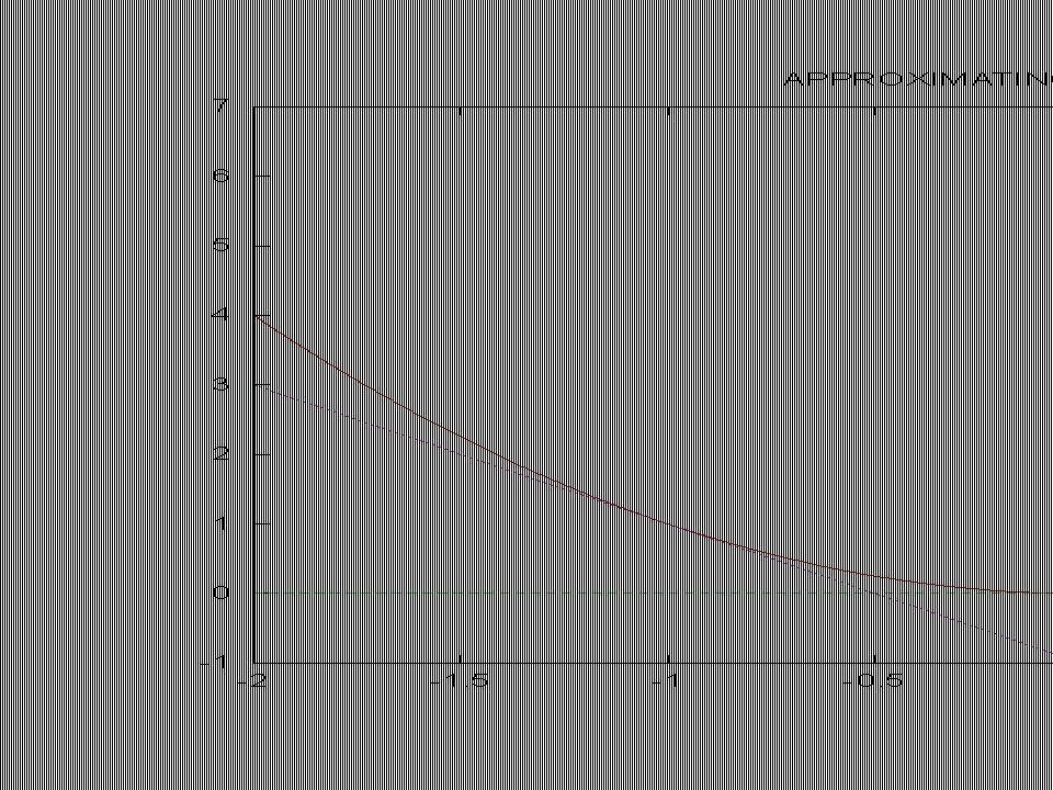
7
Approximating the Quadratic Approximate x 2 by a set of tangent lines (here x is a scalar, corresponding to x 1 in the previous slides) d(x 2 )/dx = 2x, so the tangent line at (a, a 2 ) is given by y – a 2 = 2a (x-a) or y = 2ax – a 2 The upper envelope of the tangent lines gets closer and closer to the real curve
 d(x 2 )/dx = 2x, so the tangent line at (a, a 2 ) is given by y – a 2 = 2a (x-a) or y = 2ax – a 2 The upper envelope of the tangent lines gets closer and closer to the real curve")
14
Approximating the Quadratic Minimize Max {y 1, y 2, y 3, y 4, y 5, y 6, y 7 } Subject to: -x 1 + x 2 ≥ 3 -x 1 – x 2 ≥ -2 y 1 = 0 y 2 = 2x 1 – 1 y 3 = -2x 1 – 1 y 4 = 4x 1 – 4 y 5 = -4x 1 – 4 y 6 = x 1 – 0.25 y 7 = -x 1 – 0.25 Minimize (x 1 ) 2 Subject to: -x 1 + x 2 ≥ 3 -x 1 – x 2 ≥ -2
 2 Subject to: -x 1 + x 2 ≥ 3 -x 1 – x 2 ≥ -2")
15
Approximating the Quadratic Minimize z Subject to: -x 1 + x 2 ≥ 3 -x 1 – x 2 ≥ -2 z ≥ 0 z ≥ 2x 1 – 1 z ≥ -2x 1 – 1 z ≥ 4x 1 – 4 z ≥ -4x 1 – 4 z ≥ x 1 – 0.25 z ≥ -x 1 – 0.25 Minimize (x 1 ) 2 Subject to: -x 1 + x 2 ≥ 3 -x 1 – x 2 ≥ -2
 2 Subject to: -x 1 + x 2 ≥ 3 -x 1 – x 2 ≥ -2")
16
Approximating the Quadratic Minimize z Subject to: -x 1 + x 2 ≥ 3 -x 1 – x 2 ≥ -2 z ≥ 0 z ≥ 2x 1 – 1 z ≥ -2x 1 – 1 z ≥ 4x 1 – 4 z ≥ -4x 1 – 4 z ≥ x 1 – 0.25 z ≥ -x 1 – 0.25 Minimize (x 1 ) 2 Subject to: -x 1 + x 2 ≥ 3 -x 1 – x 2 ≥ -2 LPs can give successively better approximations
 2 Subject to: -x 1 + x 2 ≥ 3 -x 1 – x 2 ≥ -2 LPs can give successively better approximations")
17
Approximating the Quadratic Minimize z Subject to: -x 1 + x 2 ≥ 3 -x 1 – x 2 ≥ -2 z ≥ 0 z ≥ 2x 1 – 1 z ≥ -2x 1 – 1 z ≥ 4x 1 – 4 z ≥ -4x 1 – 4 z ≥ x 1 – 0.25 z ≥ -x 1 – 0.25 Minimize (x 1 ) 2 Subject to: -x 1 + x 2 ≥ 3 -x 1 – x 2 ≥ -2 Quadratic Programs = Linear Programs in the “limit”
 2 Subject to: -x 1 + x 2 ≥ 3 -x 1 – x 2 ≥ -2 Quadratic Programs = Linear Programs in the limit")
18
QPs and LPs Is it necessarily true for a QP that if an optimal solution exists and a BFS exists, then an optimal BFS exists?

19
QPs and LPs Is it necessarily true for a QP that if an optimal solution exists and a BFS exists, then an optimal BFS exists? NO!! Intuition: When we think of a QP as being approximated by a succession of LPs, we have to add many new variables and constraints; the BFS of the new LP may not be the same as the BFS of the feasible region for the original constraints.

20
QPs and LPs In any QP, it is still true that any local minimum is also a global minimum Is it still true that the average of two feasible solutions is also feasible?

21
QPs and LPs In any QP, it is still true that any local minimum is also a global minimum Is it still true that the average of two feasible solutions is also feasible? – Yes!!

22
QPs and LPs In any QP, it is still true that any local minimum is also a global minimum Is it still true that the average of two feasible solutions is also feasible? – Yes!! QPs still have enough nice structure that they are easy to solve

23
Formal Definition of a QP Minimize c T x + y T y s.t. Ax = b Ex ≥ f Gx ≤ h y = Dx Where x, y are decision variables. All vectors are column vectors.

24
Formal Definition of a QP Minimize c T x + y T y s.t. Ax = b Ex ≥ f Gx ≤ h y = Dx Where x, y are decision variables. All vectors are column vectors. The quadratic part is always non-negative

25
Minimize c T x + y T y s.t. Ax = b Ex ≥ f Gx ≤ h y = Dx Where x, y are decision variables. All vectors are column vectors. Formal Definition of a QP i.e. ANY LINEAR CONSTRAINTS

26
Equivalently Minimize c T x + (Dx) T (Dx) s.t. Ax = b Ex ≥ f Gx ≤ h Where x are decision variables. All vectors are column vectors.

27
Equivalently Minimize c T x + x T D T Dx s.t. Ax = b Ex ≥ f Gx ≤ h Where x are decision variables. All vectors are column vectors.

28
Equivalently Minimize c T x + x T Px s.t. Ax = b Ex ≥ f Gx ≤ h Where x are decision variables. All vectors are column vectors. P is positive semi-definite (a matrix that can be written as D T D for some D)
.")
29
Equivalently Minimize c T x + y T y s.t. Ax = b Ex ≥ f Gx ≤ h Where x are decision variables, and y represents a subset of the coordinates of x. All vectors are column vectors.

30
Equivalently Instead of minimizing, the objective function is Maximize c T x – x T Px For some positive semi-definite matrix P

31
Is this a QP? Minimize xy s.t. x + y = 5

32
Is this a QP? Minimize xy s.t. x + y = 5 No, since x = 1, y=-1 gives xy = -1. Hence xy is not an acceptable quadratic part for the objective function.

33
Is this a QP? Minimize xy s.t. x + y = 5 x, y ≥ 0

34
Is this a QP? Minimize xy s.t. x + y = 5 x, y ≥ 0 No, for the same reason as before!

35
Is this a QP? Minimize x 2 -2xy + y 2 - 2x s.t. x + y = 5

36
Is this a QP? Minimize x 2 -2xy + y 2 - 2x s.t. x + y = 5 Yes, since we can write the quadratic part as (x- y)(x-y).
(x-y)..")
37
A Useful Fact If P and Q are positive semi-definite, then so is P + Q

38
An example: Linear Regression Let f be an unknown real-valued function defined on points in d dimensions. We are given the value of f on K points, x 1,x 2, …,x K, where each x i is d × 1 f(x i ) = y i Goal: Find the best linear estimator of f Linear estimator: Approximate f(x) as x T p + q – p and q are decision variables, (p is d × 1, q is scalar) Error of the linear estimator for x i is denoted Δ i Δ i = (x i ) T p + q - y i
 = y i Goal: Find the best linear estimator of f Linear estimator: Approximate f(x) as x T p + q – p and q are decision variables, (p is d × 1, q is scalar) Error of the linear estimator for x i is denoted Δ i Δ i = (x i ) T p + q - y i.")
39
Linear Regression Best linear estimator: one which minimizes the error – Individual error for x i : Δ i – Overall error: commonly used formula is the sum of the squares of the individual errors

40
Linear Least Squares Regression QP: Minimize Σ i (Δ i ) 2 s.t. For all i in {1..K}: Δ i = (x i ) T p + q - y i
 T p + q - y i.")
41
Linear Least Squares Regression QP: Minimize Σ i (Δ i ) 2 s.t. For all i in {1..K}: Δ i = (x i ) T p + q - y i Can simplify this further.
 T p + q - y i Can simplify this further..")
42
Linear Least Squares Regression QP: Minimize Σ i (Δ i ) 2 s.t. For all i in {1..K}: Δ i = (x i ) T p + q - y i Can simplify this further. Let X denote the d × K matrix obtained from all the x i ’s: X = (x 1 x 2 … x K )
 T p + q - y i Can simplify this further. Let X denote the d × K matrix obtained from all the x i ’s: X = (x 1 x 2 … x K ).")
43
Linear Least Squares Regression QP: Minimize Σ i (Δ i ) 2 s.t. For all i in {1..K}: Δ i = (x i ) T p + q - y i Can simplify this further. Let X denote the d × K matrix obtained from all the x i ’s: X = (x 1 x 2 … x K ) Let e denote a K × 1 vector of all 1’s
 T p + q - y i Can simplify this further. Let X denote the d × K matrix obtained from all the x i ’s: X = (x 1 x 2 … x K ) Let e denote a K × 1 vector of all 1’s.")
44
Linear Least Squares Regression QP: Minimize Δ T Δ s.t. Δ = X T p + qe – y

45
Simple Portfolio Optimization Consider a market with N financial products (stocks, bonds, currencies, etc.) and M future market scenarios Payoff matrix P: P i,j = Payoff from product j in the i-th scenario x j = # of units bought of j-th product c j = cost per unit of j-th product Additional assumption: Probability q i of market scenario i happening is given
 and M future market scenarios Payoff matrix P: P i,j = Payoff from product j in the i-th scenario x j = # of units bought of j-th product c j = cost per unit of j-th product Additional assumption: Probability q i of market scenario i happening is given")
46
Simple Portfolio Optimization Example: Stock mutual fund and bond mutual fund, each costing $1, with two scenarios, occurring with 50% probability each: that the economy will grow next year or stagnate PAYOFF MATRIX STOCKBOND GROWTH0.30.05 STAGNATION-0.10.05

47
Simple Portfolio Optimization Example: Stock mutual fund and bond mutual fund, each costing $1, with two scenarios, occurring with 50% probability each: that the economy will grow next year or stagnate PAYOFF MATRIX STOCKBOND GROWTH0.30.05 STAGNATION-0.10.05 What portfolio maximizes expected payoff? 100% STOCK, 50% EACH, 100% BOND

48
Simple Portfolio Optimization Example: Stock mutual fund and bond mutual fund, each costing $1, with two scenarios, occurring with 50% probability each: that the economy will grow next year or stagnate PAYOFF MATRIX STOCKBOND GROWTH0.30.05 STAGNATION-0.10.05 What portfolio maximizes expected payoff? 100% STOCK, 50% EACH, 100% BOND

49
Simple Portfolio Optimization Example: Stock mutual fund and bond mutual fund, each costing $1, with two scenarios, occurring with 50% probability each: that the economy will grow next year or stagnate PAYOFF MATRIX STOCKBOND GROWTH0.30.05 STAGNATION-0.10.05 What portfolio minimizes variance? 100% STOCK, 50% EACH, 100% BOND

50
Simple Portfolio Optimization Example: Stock mutual fund and bond mutual fund, each costing $1, with two scenarios, occurring with 50% probability each: that the economy will grow next year or stagnate PAYOFF MATRIX STOCKBOND GROWTH0.30.05 STAGNATION-0.10.05 What portfolio minimizes variance? 100% STOCK, 50% EACH, 100% BOND

51
Simple Portfolio Optimization Example: Stock mutual fund and bond mutual fund, each costing $1, with two scenarios, occurring with 50% probability each: that the economy will grow next year or stagnate PAYOFF MATRIX STOCKBOND GROWTH0.30.05 STAGNATION-0.10.05 What portfolio minimizes variance subject to getting at least 7.5% expected returns? 100% STOCK, 50% EACH, 100% BOND

52
Simple Portfolio Optimization Example: Stock mutual fund and bond mutual fund, each costing $1, with two scenarios, occurring with 50% probability each: that the economy will grow next year or stagnate PAYOFF MATRIX STOCKBOND GROWTH0.30.05 STAGNATION-0.10.05 What portfolio minimizes variance subject to getting at least 7.5% expected returns? 100% STOCK, 50% EACH, 100% BOND

53
Minimizing Variance (≈ Risk) Often, we want to minimize the variance of our portfolio, subject to some cost budget b and some payoff target π Let y i denote the payoff in market scenario i y i = P i x Expected payoff= z = Σ i q i y i = q T y Variance = Σ i q i (y i - z) 2 = Σ i ((q i ) 1/2 (y i - z)) 2 Let v i denote (q i ) 1/2 (y i – z)
 Often, we want to minimize the variance of our portfolio, subject to some cost budget b and some payoff target π Let y i denote the payoff in market scenario i y i = P i x Expected payoff= z = Σ i q i y i = q T y Variance = Σ i q i (y i - z) 2 = Σ i ((q i ) 1/2 (y i - z)) 2 Let v i denote (q i ) 1/2 (y i – z)")
54
Portfolio Optimization: QP Minimize v T v s.t. c T x ≤ b y = Px z = q T y z ≥ π (for all i in {1…K}): v i = (q i ) 1/2 (y i – z)
: v i = (q i ) 1/2 (y i – z).")
55
THANK YOU!!!

Similar presentations


 of a function of variables, known as ‘objective function’,>")

 (Chap.29)>")


