1. Chapter 9 Quantitative Genetics
Traits such as cystic fibrosis or flower color in peas produce distinct phenotypes that are readily distinguished.
Such discrete traits, which are determined by a single gene, are the minority in nature.
Most traits are determined by the effects of multiple genes.

2. Continuous Variation
Traits determined by many genes show continuous variation.
Examples in humans include height, intelligence, athletic ability, skin color.
Beak depth in Darwin’s finches and beak length in soapberry bugs also show continuous variation.

4. Quantitative Traits
For continuous traits we cannot assign individuals to discrete categories. Instead we must measure them.
Therefore, characters with continuously distributed phenotypes are called quantitative traits.

5. Quantitative Traits
Quantitative traits determined by influence of (1) genes and (2) environment.

6. East’s 1916 work on quantitative traits
In early 20th century debate over whether Mendelian genetics could explain continuous traits.
Edward East (1916) showed it could.
Studied longflower tobacco (Nicotiana longiflora)

7. East’s 1916 work on quantitative traits
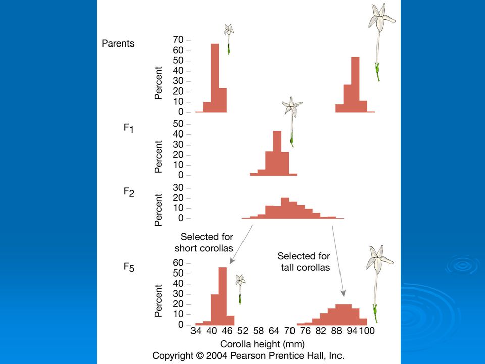
East studied corolla length (petal part of flower) in tobacco.
Crossed pure breeding short and long corolla individuals to produce F1 generation. Crossed F1’s to create F2 generation.

8. East’s 1916 work on quantitative traits
Using Mendelian genetics we can predict expected character distributions if character determined by one gene, two genes, or more etc.
(You need to understand how to do Punnett Squares)

11. East’s 1916 work on quantitative traits
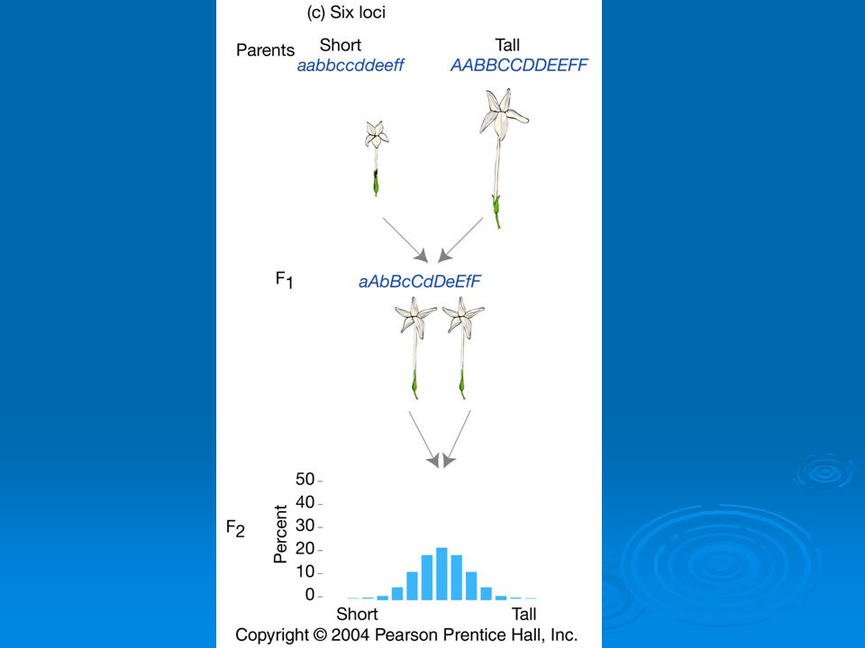
Depending on number of genes, models predict different numbers of phenotypes.
One gene: 3 phenotypes
Two genes: 5 phenotypes
Six genes: 13 phenotypes. Continuous distribution.

12. East’s 1916 work on quantitative traits
How do we decide if a quantitative trait is under the control of many genes?
In one- and two-locus models many F2 plants have phenotypes like the parental strains.
Not so with 6-locus model. Just 1 in 4,096 individuals will have the genotype aabbccddeeff.

13. East’s 1916 work on quantitative traits
But, if Mendelian model works you should be able to recover the parental phenotypes through selective breeding.
East selectively bred for both short and long corollas. By generation 5 most plants had corolla lengths within the range of the original parents.

15. East’s 1916 work on quantitative traits
Plants in F5 generation of course were not exactly the same size as their ancestors even though they were genetically identical.
Why?

16. East’s 1916 work on quantitative traits
Environmental effects.
Because of environmental differences genetically identical organisms may differ greatly in phenotype.

17. Genetically identical plants
grown at different elevations
differ enormously
(Clausen et al. 1948)

18. Skip section 9.2 QTL mapping

19. Measuring Heritable Variation
People differ in many traits e.g. height.
Is height heritable?

20. Measuring Heritable Variation
A person’s height is determined by their genes operating within their environment.
A woman who is 5 feet tall did not get four feet of her height from her genes and a foot of height from her environment.
It is important to realize that her height resulted from her genes operating within her environment.

21. Measuring Heritable Variation
How can we disentangle the effects of genes and environment?
We can’t do it by looking at one individual. But we can ask for example is the smallest woman in our distribution shorter than the tallest woman because they have
(i) different genes
(ii) grew up in different environments or
(iii) both

22. Measuring Heritable Variation
In practice what population geneticists try to do is to figure out what fraction of variation in a trait is due to variation in genes and what fraction is due to variation in environmental conditions.
The fraction of total variation in a trait that is due to variation in genes is called the heritability of a trait.

23. Measuring Heritable Variation
Heritability is often misinterpreted as the extent to which the phenotype is determined by the genotype or by the genes inherited from the parent.
This is not correct because many loci are fixed and so do not contribute to variation. A locus can affect a trait even if it is not variable.
The fact that humans have two eyes is genetically determined, but heritability of eye number is zero.

24. Measuring Heritable Variation
Definition: Heritability measures what fraction of variation in a trait (e.g. height) is due to variation in genes and what fraction is due to variation in environment.
Heritability estimates are based on population data.

25. Measuring Heritable Variation
Total variation in trait is phenotypic variation Vp.
Variation among individuals due to their genes is genetic variation Vg
Variation among individuals due to their environment is environmental variation Ve.

26. Measuring Heritable Variation
Heritability symbolized by H2 = Vg/Vp
H2 = Vg/Vp
Because Vp=Vg+Ve
H2 = Vg/Vg+Ve
H2 is broad-sense heritability. Heritability always a number between 0 and 1.

27. Estimating heritability from parents and offspring
If variation among individuals is due at least in part to variation in genes then offspring will resemble their parents.
Can assess this relationship using scatter plots.

28. Estimating heritability from parents and offspring
The midparent value (average of the two parents) is regressed against offspring value and a best fit line is determined.
The slope of the relationship is the change in the y variable per unit change in the x variable.

29. Estimating heritability from parents and offspring
If offspring don’t resemble parents then best fit line has a slope of approximately zero.
Slope of zero indicates most variation in individuals due to variation in environments.

31. Estimating heritability from parents and offspring
If offspring strongly resemble parents then best fit line slope will be close to 1.

33. Estimating heritability from parents and offspring
Most traits in most populations fall somewhere in the middle with offspring showing moderate resemblance to parents.

36. Estimating heritability from parents and offspring
Slope of best fit line is between 0 and 1.
Slope of a regression line represents narrow-sense heritability (h2).

37. Narrow-sense heritability
Narrow-sense heritability distinguishes between two components of genetic variation:
Va additive genetic variation: variation due to additive effects of genes.
Vd dominance genetic variation: variation due to gene interactions such as dominance and epistasis.

38. Narrow-sense heritability
h2 = Va/(Va + Vd + Ve)

39. Narrow-sense heritability
When estimating heritability important to remember parents and offspring share environment.
To make sure there is no correlation between environments experienced by parents and offspring requires cross-fostering experiments.

40. Smith and Dhondt (1980)
Smith and Dhondt (1980) studied heritability of beak size in Song Sparrows.
Moved eggs and young to nests of foster parents. Compared chicks’ beak dimensions to parents and foster parents.

43. Smith and Dhondt (1980)
Smith and Dhondt estimated heritability of bill depth about 0.98.

44. Estimating heritability from twins
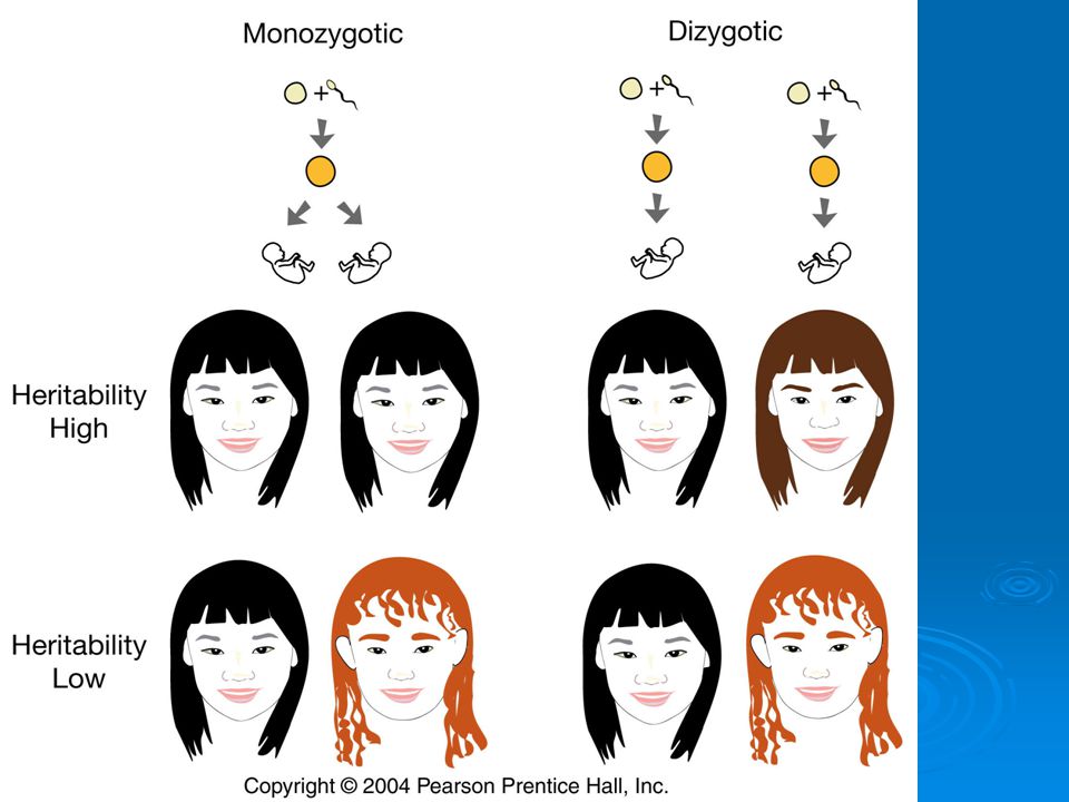
Monozygotic twins are genetically identical dizygotic are not.
Studies of twins can be used to assess relative contributions of genes and environment to traits.

46. McClearn et al.’s (1997) twin study
McClearn et al. (1997) used twin study to assess heritability of general cognitive ability.
Studied 110 pairs of monozygotic [“identical” twins i.e. derived from splitting of one egg] and 130 pairs of dizygotic twins in Sweden.

47. McClearn et al.’s (1997) twin study
All twins at least 80 years old, so plenty of time for environment to exert its influence.
However, monozygotic twins resembled each other much more than dizygotic.
Estimated heritability of trait at about 0.62.

48. Measuring differences in survival and reproduction
Heritable variation in quantitative traits is essential to Darwinian natural selection.
Also essential is that there are differences in survival and reproductive success among individuals. Need to be able to measure this.

49. Measuring differences in survival and reproduction
Need to be able to quantify difference between winners and losers in trait of interest. This is strength of selection.

50. Measuring differences in survival and reproduction
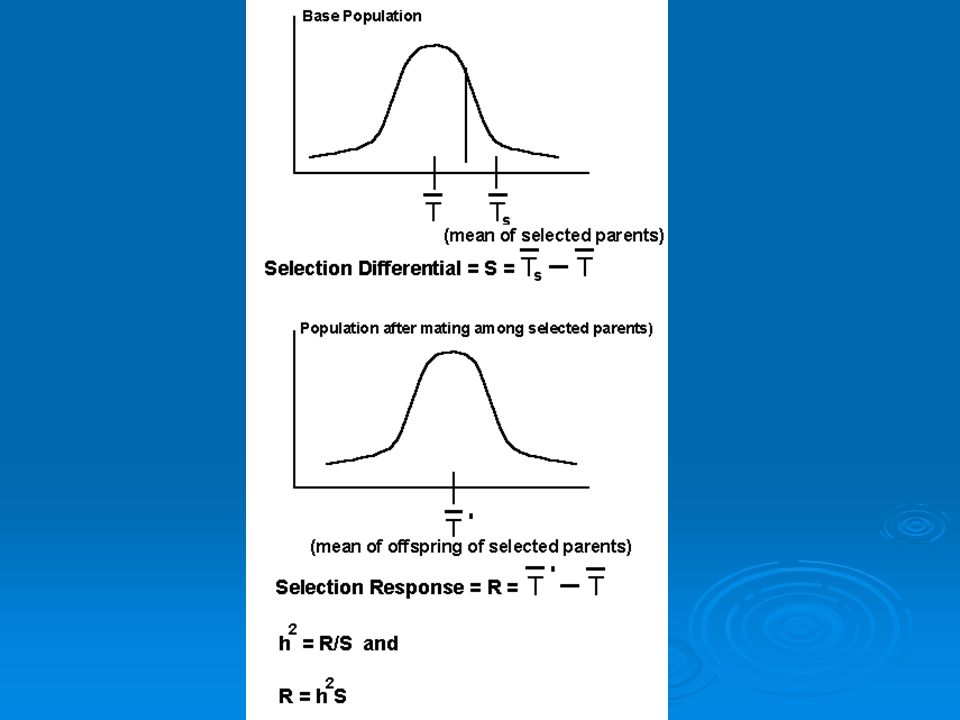
If some animals in a population breed and others don’t and you compare mean values of some trait (say mass) for the breeders and the whole population, the difference between them (and one measure of the strength of selection) is the selection differential (S).
This term is derived from selective breeding trials.

53. Measuring differences in survival and reproduction
Another way to assess selection differential is to use linear regression.
To do this we can regress fitness against the value of a phenotypic trait.
Slope of best-fit line is the selection differential.

54. Evolutionary response to selection
Knowing heritability and selection differential we can predict evolutionary response to selection (R).
This is how much of a change in a trait value we expect to see from one generation to the next.
Given by formula: R=h2S
R is predicted response to selection, h2 is heritability, S is selection differential.

56. Alpine skypilots and bumble bees
Alpine skypilot perennial wildflower found in the Rocky Mountains.
Populations at timberline and tundra differed in size. Tundra flowers about 12% larger in diameter.
Timberline flowers pollinated by many insects, but tundra only by bees. Bees known to be more attracted to larger flowers.

57. Alpine skypilots and bumble bees
Candace Galen (1996) wanted to know if selection by bumblebees was responsible for larger size flowers in tundra and, if so, how long it would take flowers to increase in size by 12%.

58. Alpine skypilots and bumble bees
First, Galen estimated heritability of flower size. Measured plants flowers, planted their seeds and (seven years later!) measured flowers of offspring.
Concluded % of variation in flower size was heritable (h2).

59. Alpine skypilots and bumble bees
Next, she estimated strength of selection by bumblebees by allowing bumblebees to pollinate a caged population of plants, collected seeds and grew plants from seed.
Correlated number of surviving young with flower size of parent. Estimated selection gradient at 0.13 and the selection differential (S) at 5% (successfully pollinated plants 5% larger than population average).

60. Alpine skypilots and bumble bees
Using her data Galen predicted response to selection R.
R=h2S
R=0.2*0.05 = 0.01 (low end estimate)
R=1.0*0.05 = 0.05 (high end estimate)

61. Alpine skypilots and bumble bees
Thus, expect 1-5% increase in flower size per generation.
Difference between populations in flower size plausibly due to bumblebee selection pressure.

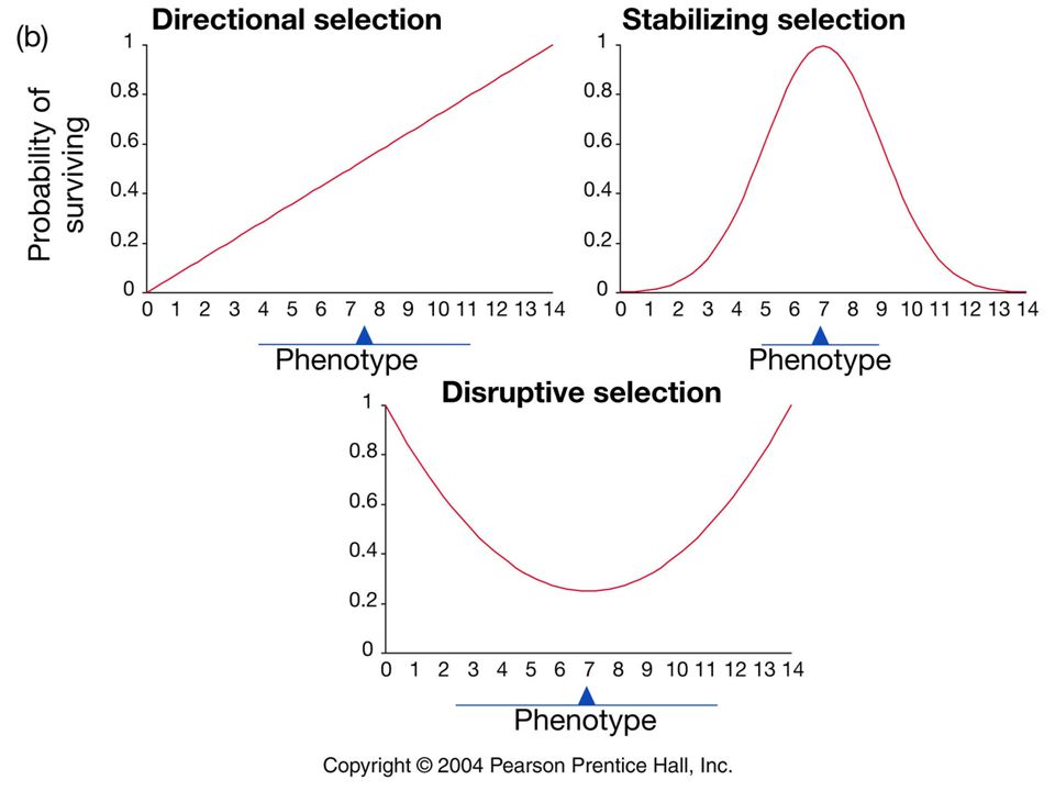
62. Modes of selection Three majors modes of selection recognized.
Directional
Stabilizing
Disruptive

63. Directional selection
In directional selection fitness increases or decreases with the value of a trait.

65. Directional selection
E.g bumblebees and Alpine skypilots. Flower size increases under bumble bee selection.
Darwin’s finches beak size increased during drought

66. Stabilizing Selection
In stabilizing selection individuals with intermediate values of a trait are favored.

68. Stabilizing Selection
Weis and Abrahamson (1986) studied fly Eurosta solidaginis.
Female lays eggs on goldenrod and larva forms a gall for protection.
Two dangers for larva Galls parasitized by wasps and 2. birds open galls and eat larva.

69. Stabilizing selection
Parasitoid wasps impose strong directional selection on wasps favoring larger gall size.

71. Stabilizing selection
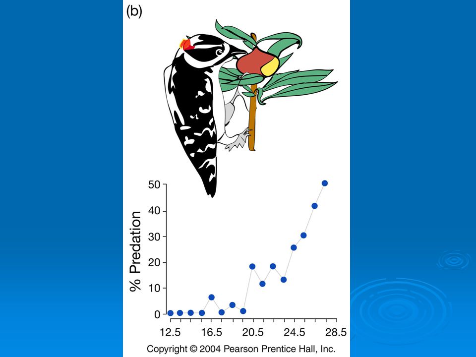
Birds impose strong directional selection favoring smaller gall size

73. Stabilizing selection
Net result of selection by birds and wasps operating in opposite directions is stabilizing selection.

75. Disruptive selection
In disruptive selection individuals with extreme values of a trait are favored.

77. Disruptive selection
Bates Smith (1993) studied black-bellied seedcrackers.
Birds in population have one of two distinct bill sizes.

78. Disruptive selection
Bates Smith found that among juveniles, individuals with beaks of intermediate size did not survive.