Download presentation
Presentation is loading. Please wait.

1
Introduction Process Simulation

2
Classification of the models
Black box – white box Black box – know nothing about process in apparatus, only dependences between inputs and outputs are established. Practical realisation of Black box is the neural network White box – process mechanism is well <??> known and described by system of equations

3
Classification of the models
Deterministic – Stochastic Deterministic – for one given set of inputs only one set of outputs is calculated with probability equal 1. Stochastic – random phenomenon affects on process course (e.g. weather), output set is given as distribution of random variables
, output set is given as distribution of random variables.")
4
Classification of the models
Microscopic- macroscopic Microscopic – includes part of process or apparatus Macroscopic – includes whole process or apparatus

5
Elements of the model Balance dependences Based upon basic nature laws
of conservation of mass of conservation of energy of conservation of atoms number of conservation of electric charge, etc. Balance equation (for mass): (overall and for specific component without reaction) Input – Output = Accumulation or (for specific component if chemical reactions presents) Input – Output +Source = Accumulation
: (overall and for specific component without reaction) Input – Output = Accumulation or (for specific component if chemical reactions presents) Input – Output +Source = Accumulation.")
6
Elements of the model Constitutive equations
Newton eq. – for viscous friction Fourier eq. – for heat conduction Fick eq. – for mass diffusion

7
Elements of the model Phase equilibrium equations – important for mass transfer Physical properties equations – for calculation parameters as functions of temperature, pressure and concentrations. Geometrical dependences – involve influence of apparatus geometry on transfer coefficients – convectional streams.

8
Structure of the simulation model
Structure corresponds to type of model equations Structure depends on: Type of object work: Continuous, steady running Periodic, unsteady running Distribution of parameters in space Equal in every point of apparatus – aggregated parameters (butch reactor with ideal mixing) Parameters are space dependent– displaced parameters
 Parameters are space dependent– displaced parameters.")
9
Structure of the model Steady state Unsteady state
Aggregated parameters Algebraic eq. Ordinary differential eq. Displaced parameters Differential eq. Ordinary for 1- dimensional case Partial for 2&3- dimensional case (without time derivative, usually elliptic) Partial differential eq. (with time derivative, usually parabolic)
 Partial differential eq. (with time derivative, usually parabolic)")
10
Process simulation the act of representing some aspects of the industry process (in the real world) by numbers or symbols (in the virtual world) which may be manipulated to facilitate their study. Facilitate - ułatwiać
 by numbers or symbols (in the virtual world) which may be manipulated to facilitate their study. Facilitate - ułatwiać.")
11
Process simulation (steady state)
Flowsheeting problem Specification (design) problem Optimization problem Synthesis problem by Rafiqul Gani
 problem. Optimization problem. Synthesis problem. by Rafiqul Gani.")
12
Flowsheeting problem Given: To calculate: All of the input information
All of the operating condition All of the equipment parameters To calculate: All of the outputs FLOWSHEET SCHEME INPUT OPERATING CONDITIONS EQUIPMENT PARAMETERS PRODUCTS

13
R.Gani

14
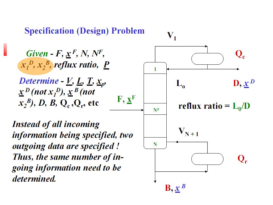
Specyfication problem
FLOWSHEET SCHEME INPUT OPERATING CONDITIONS EQUIPMENT PARAMETERS PRODUCTS Given: Some input & some output information Some operating condition Some equipment parameters To calculate: Undefined inputs&outputs Undefined operating condition Undefined equipment parameters

15
Specyfication problem
NOTE: degree of freedom is the same as in flowsheeting problem.

17
Assume value to be guessed: D, Qr
Given: feed composition and flowrates, target product composition Assume value to be guessed: D, Qr Find: product flowrates, heating duties Solve the flowsheeting problem Adjust D, Qr Is target product composition satisfied ? STOP

18
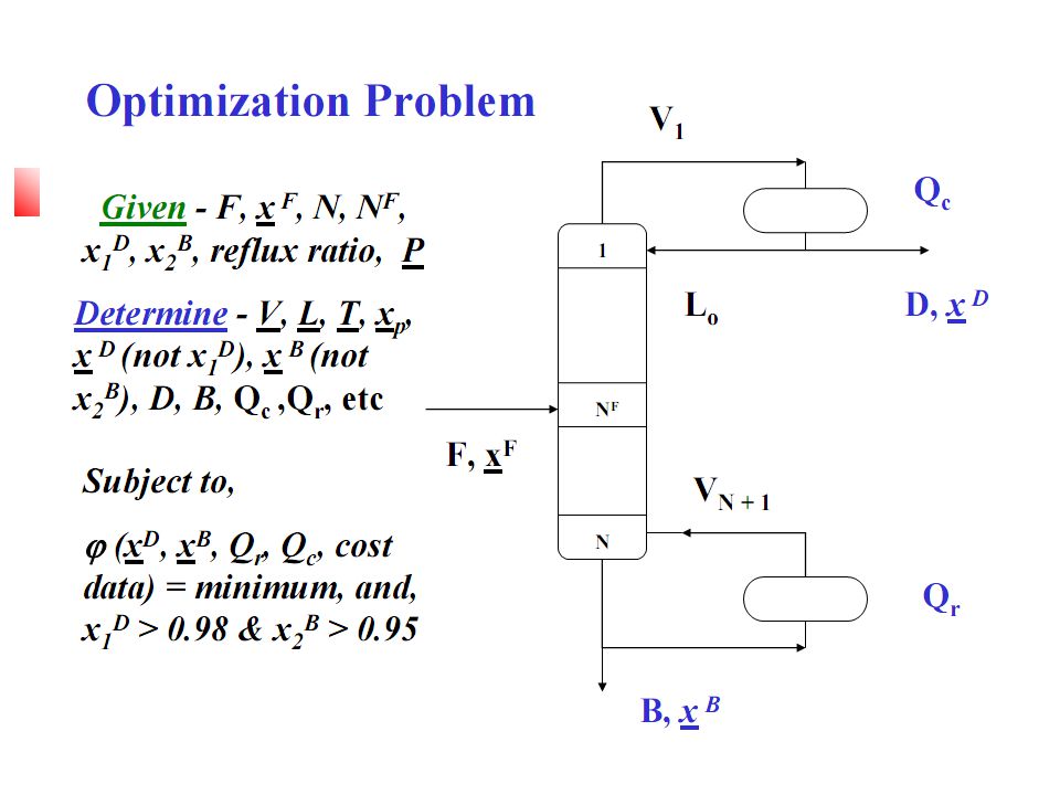
Process optimisation the act of finding the best solution (minimize capital costs, energy... maximize yield) to manage the process (by changing some parameters, not apparatus)
 to manage the process (by changing some parameters, not apparatus)")
20
Assume value to be guessed: D, Qr
Given: feed composition and flowrates, target product composition Assume value to be guessed: D, Qr Find: product flowrate, heating duty Solve the flowsheeting problem Adjust D, Qr Is target product composition satisfied AND =min. STOP

21
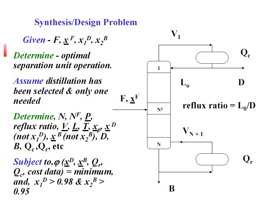
Process synthesis/design problem
the act of creation of a new process. Given: inputs (some feeding streams can be added/changed latter) Outputs (some byproducts may be unknown) To find: Flowsheet (topology) equipment parameters operations conditions
 Outputs (some byproducts may be unknown) To find: Flowsheet (topology) equipment parameters. operations conditions.")
22
Process synthesis/design problem
flowsheet undefined INPUT OUTPUT

24
Assume value to be guessed: D, Qr, N, NF, R/D etc.
Given: feed composition and flowrates, target product composition Assume value to be guessed: D, Qr, N, NF, R/D etc. Find: product flowrate, heating duty, column param. etc. Solve the flowsheeting problem Adjust D, Qr As well as N, NF, R/D etc. Is target product composition satisfied AND =min. STOP

25
Process simulation - why?
COSTS Material – easy to measure Time – could be estimated Risc – hard to measure and estimate

26
Modelling objects in chemical and process engineering
Unit operation Process build-up on a few unit operations

27
Software for process simulation
Universal software: Worksheets – Excel, Calc (Open Office) Mathematical software – MathCAD, Matlab Specialized software – process simulators. Equipped with: Data base of apparatus models Data base of components and mixtures properties Solver engine User friendly interface
 Mathematical software – MathCAD, Matlab. Specialized software – process simulators. Equipped with: Data base of apparatus models. Data base of components and mixtures properties. Solver engine. User friendly interface.")
28
Software process simulators (flawsheeting programs)
Started in early 70’ At the beginning dedicated to special processes Progress toward universality Some actual process simulators: ASPEN Tech /HYSYS ChemCAD PRO/II ProSim Design II for Windows

29
Chemical plant system The apparatus set connected with material and energy streams. Most contemporary systems are complex, i.e. consists of many apparatus and streams. Simulations can be use during: Investigation works – new technology Project step – new plants (technology exists), Runtime problem identification/solving – existing systems (technology and plant exists) test
, Runtime problem identification/solving – existing systems (technology and plant exists) test.")
30
Chemical plant system characteristic parameters can be specified for every system separately according to: Material streams Apparatus

31
Apparatus-streams separation
Assumption: All processes (chemical reaction, heat exchange etc.) taking places in the apparatus and streams are in the chemical and thermodynamical equilibrium state. Why separate? It’s make calculations easier
 taking places in the apparatus and streams are in the chemical and thermodynamical equilibrium state. Why separate It’s make calculations easier.")
32
Streams parameters Flow rate (mass, volume, mol per time unit)
Composition (mass, volume, molar fraction) Temperature Pressure Vapor fraction Enthalpy
 Temperature. Pressure. Vapor fraction. Enthalpy.")
33
Streams degrees of freedom
DFs=NC+2 e.g.: NC=2 -> DFs=4 Assumed: F1, F2, T, P Calculated: enthalpy vapor fraction

34
Apparatus parameters & DF
Characteristics for each apparatus type. E.g. heat exchanger : Heat exchange area, A [m2] Overall heat-transfer coefficient, U (k) [Wm-2K-1] Log Mean Temperature Difference, LMTD [K] degrees of freedom are unique to equipment type
 [Wm-2K-1] Log Mean Temperature Difference, LMTD [K] degrees of freedom are unique to equipment type.")
35
Types of flowsheeting calculation
Steady state calculation Dynamic calculation

36
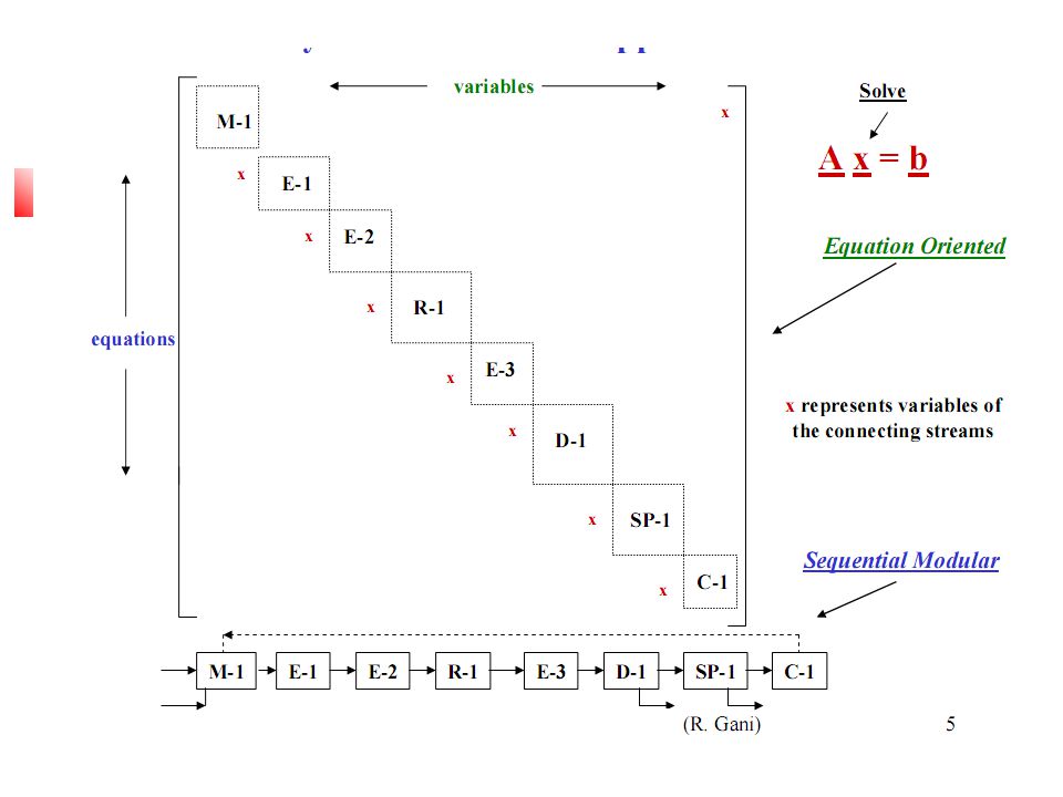
Calculation subject Number of equations of mass and energy balance for entire system Can be solved in two ways:

38
Types of balance calculation
Overall balance (without use of apparatus mathematical model) Detailed balance on the base of apparatus model
 Detailed balance on the base of apparatus model.")
39
Overall balance Apparatus is considered as a black box
Needs more stream data User could not be informed about if the process is physically possible to realize.

40
Overall balance – Example
1 2 4 3 Countercurrent, tube-shell heat exchanger Given three streams data: 1, 2, 3 hence parameters of stream 4 can be easily calculated from the balance equation. DF=5 There is possibility that calculated temp. of stream 4 can be higher then inlet temp. of heating medium (stream 1).
.")
41
Overall balance – Example
1, mB 2 4 3, mA Given: mA=10kg/s mB=20kg/s t1= 70°C t2=40°C t3=20°C cpA=cpB=idem At first sight – na pierwszy rzut oka

42
Apparatus model involved
Process is being described with use of modeling equations (differential, dimensionless etc.) Only physically acceptable processes taking place Less stream data required (smaller DF number) Heat exchange example: given data for two streams, the others can be calculated from a balance and heat exchange model equations
 Only physically acceptable processes taking place. Less stream data required (smaller DF number) Heat exchange example: given data for two streams, the others can be calculated from a balance and heat exchange model equations.")
43
Loops and cut streams Loops occur when: To solve:
some products are returned and mixed with input streams when output stream heating (cooling) inputs some input (also internal) data are undefined To solve: one stream inside the loop has to be cut (tear stream) initial parameters of cut stream have to be defined Calculations have to be repeated until cut streams parameters are converted.
 inputs. some input (also internal) data are undefined. To solve: one stream inside the loop has to be cut (tear stream) initial parameters of cut stream have to be defined. Calculations have to be repeated until cut streams parameters are converted.")
44
Loops and cut streams

45
Simulation of system with heat exchanger using MathCAD

46
I.Problem definition Simulate system consists of: Shell-tube heat exchanger, four pipes and two valves on output pipes. Parameters of input streams are given as well as pipes, heat exchanger geometry and valves resistance coefficients. Component 1 and 2 are water. Pipe flow is adiabatic. Find such a valves resistance to satisfy condition: both streams output pressures equal 1bar.

47
II. Flawsheet s6 s1 1 2 3 4 6 7 5 s2 s3 s4 s5 s7 s8 s9 s10

48
Numerical data: Stream s1 Ps1 =200kPa, ts1 = 85°C, f1s1 = 10000kg/h

49
Equipment parameters:
L1=7m d1=0,025m L2=5m d2=0,16m, s=0,0016m, n=31... L3=6m, d3=0,05m z4=50 L5=7m d5=0,05m L6=10m, d6=0,05m z7=40

50
III. Stream summary table
Uknown:Ts2, Ts3, Ts4, Ts5, Ts7, Ts8, Ts9, Ts10, Ps2, Ps3, Ps4, Ps5, Ps7, Ps8, Ps9, Ps10, f1s2, f1s3, f1s4, f1s5, f2s7, f2s8, f2s9, f2s10 number of unknown variables: 26 WE NEED 26 INDEPENDENT EQUATIONS.

51
Equations from equipment information
f1s2= f1s1 f1s7= f1s6 f1s3= f1s2 f1s8= f1s7 f1s4= f1s3 f1s9= f1s8 f1s5= f1s4 f1s10= f1s9 14 equations. Still do define 26-14=12 equations

52
Heat balance equations
New variable: Q Still to define: =11 equations

53
Heat exchange equations
New variables: k, DTm: number of equations to find =11

54
Heat exchange equations
Two new variables: aT and aS number of equations to find: =12

55
Heat exchange equations
Three new variables: NuT, NuS, deq, number of equations to find: =12

56
Heat exchange equations

57
Heat exchange equations
Two new variables ReT and ReS, number of equations to find: =10

58
Pressure drop

59
Pressure drop Two new variables Re1 and l1,
number of equations to find: =9

60
Pressure drop One new variables and l2T,
number of equations to find: 9+1-3=7

61
Pressure drop Two new variables Re3 and l3,
number of equations to find: 7+2-3=6

62
Pressure drop Number of equations to find: 6-1=5

63
Pressure drop Two new variables Re5 and l5,
number of equations to find: 6+2-3=4

64
Pressure drop One new variables and l2S,
number of equations to find: 4+1-3=2

65
Pressure drop Two new variables Re6 and l6,
number of equations to find: 2+2-3=1

66
Pressure drop Number of equations to find: 1-1=0 !!!!!!!!!!!!!!

67
Agents parameters Temperatures are not constant
Liquid properties are functions of temperature Density Viscosity Thermal conductivity Specyfic heat cp Prandtl number Pr

68
Agents parameters Data are usually published in the tables

69
Agents parameters Data in tables are difficult to use Solution:
Approximate discrete data by the continuous functions.

70
Approximation Approximating function
Polynomial Approximation target: find optimal parameters of approximating function Approximation type Mean-square – sum of square of differences between discrete (from tables) and calculated values is minimum.
 and calculated values is minimum.")
71
Polynomial approximation

72
The end as of yet.

Similar presentations

>")
>")


