Download presentation
Presentation is loading. Please wait.

1
Texture

2
Limitation of pixel based processing

3
Edge detection with different threshold

4
What is texture ? There is no accurate definition. It is often used to represent all the “details” in the image. (F.e, sometimes images are divided to shape + texture. In our case we refer to the texture as images or patterns with some kind of “structure”.

5
What is Texture? For example, an image has a 50% black and 50% white distribution of pixels. Three different images with the same intensity distribution, but with different textures.

6
What is texture ? (cont’) repetition stochastic both
 repetition stochastic both")
7
Texture Texture refers to the surface quality or "feel" of an object - smooth, rough, soft, etc. Textures may be actual (felt with touch - tactile) or implied (suggested by the way an artist has created the work of art -visual).
 or implied (suggested by the way an artist has created the work of art -visual)..")
8
What would we like to do with textures? Detect regions / images with textures. Classify using texture. Segmentation: divide the image into regions with uniform texture. Synthesis – given a sample of the texture, generate random images with the same texture. Compression (Especially fractals)
.")
9
Internet source for textures http://creative.gettyimages.com/source/home/h omeCreative.aspx

10
Actual Texture Texture is the tactile quality of a surface or the representation of that surface. If it is the way something feels when you touch it, it is called real texture.

11
Simulated or Implied texture Texture is what your eyes tell you about how things in the drawing would feel if you could touch them, called simulated texture. Photography is very good at translating real texture into implied or simulated texture, but painters and draftsmen can also learn to recreate the visual appearance of textures in very convincing ways.

12
OBJECT by Meret Oppenheim

13
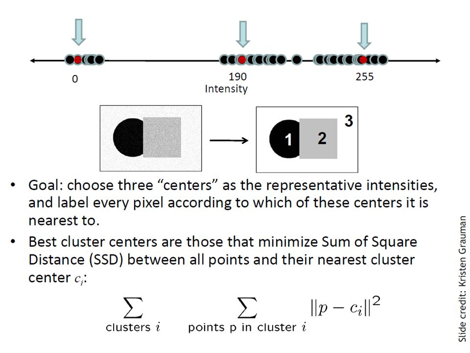
Simplest Texture Discrimination Compare histograms. –Divide intensities into discrete ranges. –Count how many pixels in each range. 0-2526-50225-25051-7576-100

14
How/why to compare Simplest comparison is SSD, many others. Can view probabilistically. –Histogram is a set of samples from a probability distribution. –With many samples it approximates distribution. –Test probability samples drawn from same distribution. Ie., is difference greater than expected when two samples come from same distribution?

15
i j k Chi-square 0.1 0.8 Chi square distance between texton histograms (Malik)
")
16
More Complex Discrimination Histogram comparison is very limiting –Every pixel is independent. –Everything happens at a tiny scale. Use output of filters of different scales.

17
What are Right Filters? Multi-scale is good, since we don’t know right scale a priori. Easiest to compare with naïve Bayes: Filter image one: (F1, F2, …) Filter image two: (G1, G2, …) S means image one and two have same texture. Approximate: P(F1,G1,F2,G2, …| S) By P(F1,G1|S)*P(F2,G2|S)*…
 Filter image two: (G1, G2, …) S means image one and two have same texture. Approximate: P(F1,G1,F2,G2, …| S) By P(F1,G1|S)*P(F2,G2|S)*….")
18
What are Right Filters? The more independent the better. –In an image, output of one filter should be independent of others. –Because our comparison assumes independence.

19
Difference of Gaussian Filters

20
Spots and Oriented Bars (Malik and Perona)
")
23
Gabor Filters Gabor filters at different scales and spatial frequencies top row shows anti-symmetric (or odd) filters, bottom row the symmetric (or even) filters.
 filters, bottom row the symmetric (or even) filters.")
24
Gabor filters are examples of Wavelets We know two bases for images: –Pixels are localized in space. –Fourier are localized in frequency. Wavelets are a little of both. Good for measuring frequency locally.

25
Markov Model Captures local dependencies. –Each pixel depends on neighborhood. Example, 1D first order model P(p1, p2, …pn) = P(p1)*P(p2|p1)*P(p3|p2,p1)*… = P(p1)*P(p2|p1)*P(p3|p2)*P(p4|p3)*…
 = P(p1)*P(p2|p1)*P(p3|p2,p1)*… = P(p1)*P(p2|p1)*P(p3|p2)*P(p4|p3)*….")
26
Markov Chains Markov Chain –a sequence of random variables – is the state of the model at time t –Markov assumption: each state is dependent only on the previous one dependency given by a conditional probability: –The above is actually a first-order Markov chain –An N’th-order Markov chain:

27
Markov Random Field A Markov random field (MRF) generalization of Markov chains to two or more dimensions. First-order MRF: probability that pixel X takes a certain value given the values of neighbors A, B, C, and D: D C X A B X X Higher order MRF’s have larger neighborhoods

28
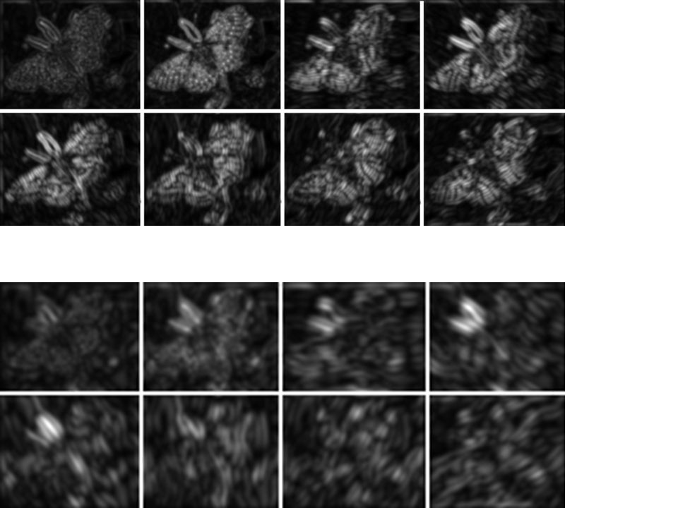
Texture Synthesis [Efros & Leung, ICCV 99] [Efros & Leung, ICCV 99] Can apply 2D version of text synthesis
![Texture Synthesis [Efros & Leung, ICCV 99] [Efros & Leung, ICCV 99] Can apply 2D version of text synthesis](http://images.slideplayer.com/12/3373821/slides/slide_28.jpg "Texture Synthesis [Efros & Leung, ICCV 99] [Efros & Leung, ICCV 99] Can apply 2D version of text synthesis")
29
Synthesizing One Pixel sample image Generated image –What is ? –Find all the windows in the image that match the neighborhood consider only pixels in the neighborhood that are already filled in –To synthesize x pick one matching window at random assign x to be the center pixel of that window SAMPLE x

30
Really Synthesizing One Pixel sample image –An exact neighbourhood match might not be present –So we find the best matches using SSD error and randomly choose between them, preferring better matches with higher probability SAMPLE Generated image x

31
Growing Texture –Starting from the initial image, “grow” the texture one pixel at a time

32
Window Size Controls Regularity

33
More Synthesis Results Increasing window size

34
More Results aluminum wire reptile skin

35
Failure Cases Growing garbageVerbatim copying

36
Image-Based Text Synthesis

37
Image Segmentation Goal: identify groups of pixels that go together

38
The Goals of Segmentation Separate image into coherent “objects”

39
The Goals of Segmentation Separate image into coherent “objects” Group together similar ‐ looking pixels for efficiency of further processing

40
Segmentation Compact representation for image data in terms of a set of components Components share “common” visual properties Properties can be defined at different level of abstractions

41
Image Segmentation

42
Introduction to image segmentation Example 1 –Segmentation based on greyscale –Very simple ‘model’ of greyscale leads to inaccuracies in object labelling

43
Introduction to image segmentation Example 2 –Segmentation based on texture –Enables object surfaces with varying patterns of grey to be segmented

44
Introduction to image segmentation

45
Example 3 –Segmentation based on motion –The main difficulty of motion segmentation is that an intermediate step is required to (either implicitly or explicitly) estimate an optical flow field –The segmentation must be based on this estimate and not, in general, the true flow
 estimate an optical flow field –The segmentation must be based on this estimate and not, in general, the true flow")
46
Introduction to image segmentation

47
Example 3 –Segmentation based on depth –This example shows a range image, obtained with a laser range finder –A segmentation based on the range (the object distance from the sensor) is useful in guiding mobile robots
 is useful in guiding mobile robots")
48
Introduction to image segmentation Original image Range image Segmented image

49
General ideas Tokens –whatever we need to group (pixels, points, surface elements, etc., etc.) Bottom up segmentation –tokens belong together because they are locally coherent Top down segmentation –tokens belong together because they lie on the same visual entity (object, scene…) > These two are not mutually exclusive
 Bottom up segmentation –tokens belong together because they are locally coherent Top down segmentation –tokens belong together because they lie on the same visual entity (object, scene…) > These two are not mutually exclusive")
50
What is Segmentation? Clustering image elements that “belong together” Partitioning – Divide into regions/sequences with coherent internal properties Grouping –Identify sets of coherent tokens in image

51
Basic ideas of grouping in human vision Gestalt properties Figure ‐ ground discrimination

52
Examples of Grouping in Vision

53
Similarity

54
Symmetry

55
Common Fate

56
Proximity

57
Gestalt Factors

58
Image Segmentation – Toy Example

Similar presentations


 Cs129 Computational Photography James Hays, Brown, Spring 2011 Many slides from Alexei Efros.>")


 Shengcai Liao, Guoying Zhao, Vili Kellokumpu,>")


.>")

