1. Visualizing the Microscopic Structure of Bilinear Data: Two components chemical systems

2. A matrix can be decomposed into the product of two significantly smaller matrices. Factorization: In many chemical studies, the measured or calculated properties of the system can be considered to be the linear sum of the term representing the fundamental effects in that system times appropriate weighing factors. D = X Y + R DX Y = + R

3. A simple one component system

4. Observing the rows of data in wavelength space

5. Observing the columns of data in time space

6. D = USV = u 1 s 11 v 1 + … + u r s rr v r Singular Value Decomposition =D U SV d 1,: d 2,: d p,: … = u 11 u 21 u p1 … s 11 v1v1 d 1,: = u 11 s 11 v 1 d 2,: = u 21 s 11 v 1 …… d p,: = u p1 s 11 v 1 For r=1 Row vectors: D = u 1 s 11 v 1

7. D = USV = u 1 s 11 v 1 + … + u r s rr v r Singular Value Decomposition [ d :,1 d :,2 … d :,q ] = u 1 s 11 [v 11 v 12 … v 1q ] d :,1 = u 1 s 11 v 11 …… d :,2 = u 1 s 11 v 12 d :,q = u 1 s 11 v 1q Column vectors: =D U SV For r=1 D = u 1 s 11 v 1

8. Rows of measured data matrix in row space: v1v1 u 11 s 11 v 1 u p1 s 11 v 1 u 11 s 11 u 21 s 11 … u p1 s 11 p points (rows of data matrix) in rows space have the following coordinates:

9. Columns of measured data matrix in column space: v 11 s 11 v 12 s 11 … v 1q s 11 q points (columns of data matrix) in columnss space have the following coordinates: u1u1 v 11 s 11 u 1 v 1q s 11 u 1

10. Visualizing the rows and columns of data matrix

11. Solutions Pure spectrum v 1j s 11 Pure conc. profile u i1 s 11

12. Two component systems

13. Visualizing data in three selected wavelengths

14. Visualizing data in three selected Times

15. Measured Data Matrix

16. D = USV = u 1 s 11 v 1 + … + u r s rr v r Singular Value Decomposition Row vectors: d 1,: d 2,: d p,: … = u 11 u 21 u p1 … s 11 v1v1 u 12 u 22 u p2 … s 22 v2v2 + d 1,: = u 11 s 11 v 1 + u 12 s 22 v 2 d 2,: = …… d p,: = u 21 s 11 v 1 + u 22 s 22 v 2 u p1 s 11 v 1 + u p2 s 22 v 2 … For r=2 D = u 1 s 11 v 1 + u 2 s 22 v 2

17. D = USV = u 1 s 11 v 1 + … + u r s rr v r Singular Value Decomposition [ d :,1 d :,2 … d :,q ] = u 1 s 11 [v 11 v 12 … v 1q ] + u 2 s 22 [v 21 v 22 … v 2q ] d :,1 = s 11 v 11 u 1 + s 22 v 21 u 2 …… d :,2 = d :,q = s 11 v 12 u 1 + s 22 v 22 u 2 s 11 v 1q u 1 + s 22 v 2q u 2 For r=2 D = u 1 s 11 v 1 + u 2 s 22 v 2 Column vectors:

18. Rows of measured data matrix in row space: u 11 s 11 d 1,: v1v1 v2v2 u 12 s 22 d 2,: d p,: u 21 s 11 u 22 s 22 u p2 s 22 u p1 s 11 … u 11 s 11 u 12 s 22 … u 21 s 11 u 22 s 22 u p1 s 11 u p2 s 22 … Coordinates of rows

19. Columns of measured data matrix in column space: u1u1 u2u2 d :, 2 d :, 1 d :, q … v 2q s 22 v 1q s 11 v 12 s 11 v 22 s 22 v 21 s 22 v 11 s 11 v 11 s 11 v 12 s 11... v 1q s 11 Coordinates of columns v 21 s 11 v 22 s 11... v 2q s 11

20. Two component chromatographic system

21. Two component Kinetic system

22. Two component multivariate calibration

23. Position of a known profile in corresponding space: dxdx T v1 T v2 v1v1 v2v2 T v1 is the length of projection of d x on v 1 vector T v1 = d x. v 1 T v2 is the length of projection of d x on v 1 vector T v2 = d x. v 2 T v1 T v2 Coordinates of d x point:

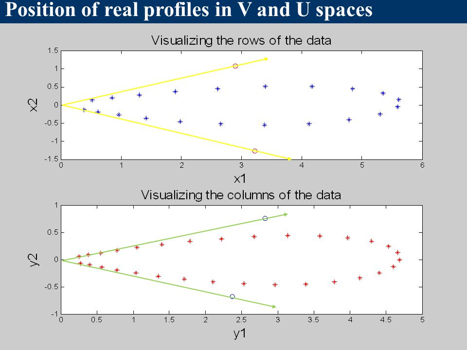
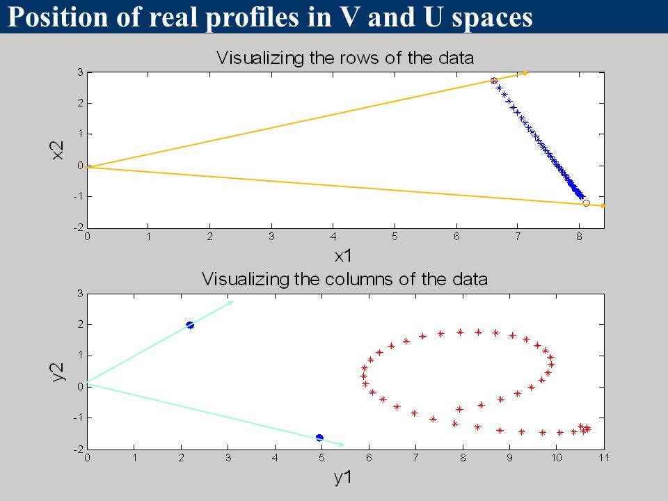
24. Position of real profiles in V and U spaces

27. Duality in Measured Data Matrix

28. p n xiTxiT xjxj x ij PpPp SnSn vnvn v1v1 vivi PnPn SpSp upup u1u1 ujuj xixi xjxj Geometrical interpretation of an n x p matrix X

29. R= C S T = U D V T = X V T R T = S C T = VD U T = Y U T X = U D = RV = U Y T V Y= V D = R T U = V X T U X YTYT U V Duality based relation between column and row spaces =

30. Non-negativity constraint and the system of inequalities: U z ≥ 0 V z ≥ 0 X = U DU= X D -1 Y = V DV= Y D -1 U z = X D -1 z ≥ 0 Hyperplanes V z = Y D -1 z ≥ 0 Hyperplanes U-space Y Points V-space X Points

31. Duality based relation between column and row spaces x i = [x i,1 x i,2 ] U i,1 z i,1 + U i,2 z i,2 … U i,N z i,N ≥ 0 The coordinates of each point in one space defines the coefficient of related hyper plane in dual space Point x in V-spaceHyper plane (D -1 x) z in U-space For two-component systems: The ith point in V-space: x i x i D -1 = [U i,1 U i,2 … U i,N ] The ith hyperplane in U-space: A point in V-space: U i,1 z 1 + U i,2 z 2 ≥ 0 A half-plane in V-space:

32. Half-plane calculation in two-component systems: General half-plane General border line can be defined for all points that the ith element of the profile is equal to zero z1z1 z2z2 0 ith half-plane ith border line General border line U i,1 z 1 + U i,2 z 2 ≥ 0 z 2 ≥ (-U i,2 /U i,1 )z 1 z 2 = (-U i,2 /U i,1 )z 1

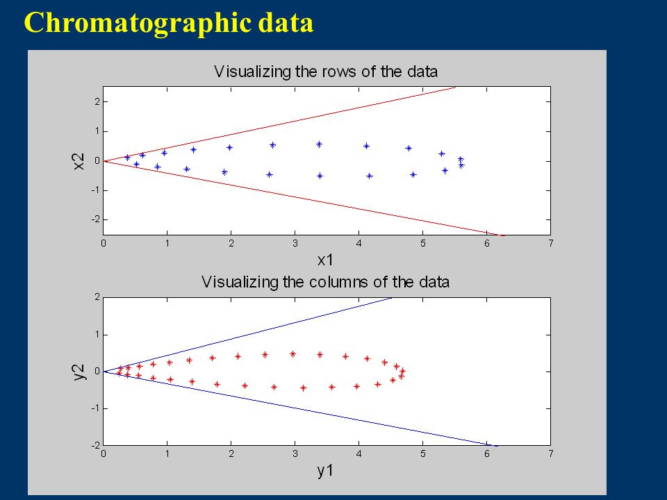
33. Chromatographic data

35. Kinetics data

37. Calibration data

39. Intensity ambiguity in V space v1v1 v2v2 a k1ak1a k2ak2a T 11 T 12 k 1 T 11 k 1 T 12 k 2 T 11 k 2 T 12

40. Normalization to unit length v1v1 v2v2 a k1ak1a k2ak2a T 11 T 12 k 1 T 11 k 1 T 12 k 2 T 11 k 2 T 12 anan a n = (1/||a||) a

41. Normalization to first eigenvector v1v1 v2v2 a k1ak1a k2ak2a T 11 T 12 k 1 T 11 k 1 T 12 k 2 T 11 k 2 T 12 1 a n = (1/(v.a))a anan

42. v1v1 v2v2 1 2 4 3 5 1’2’3’ 4’ 5’ Normalization to unit length

43. v1v1 v2v2 1 1 2 4 3 5 a = T 1 v 1 + T 2 v 2 a’ = v 1 + T v 2 1’2’3’ 4’ 5’ Normalization to first eigenvector

44. Chromatographic data- Normalized to unit length

45. Chromatographic data- Normalized to 1th eigenvector

46. Kinetics data- Normalized to unit length

47. Kinetics data- Normalized to 1th eigenvector

48. Multivariate calibration data- Normalized to unit length

49. Multivariate calibration data- Normalized to 1th eigenvector

50. The normalized abstract space of two component systems is one dimensional Data points region One dimensional normalized space There are 4 critical points in normalized abstract space of two-component systems: 1212 First inner point Second inner point First outer point Second outer point The 4 critical points can be calculated very easily and so the complete resolving of two component systems is very simple First feasible region Second feasible region Lawton-Sylvester Plot

51. Microscopic Observation of Two Component systems using Lawton- Sylvester Plot

52. First feasible solutions Second feasible solutions General Microscopic Structures of Two-Component Systems Second feasible solutions Case I) Case II) Case III)

53. Lawton-Sylvester Plot- Multivariate calibration

54. Feasible Bands- Multivariate calibration

55. Feasible Bands- Chromatographic Data

56. Feasible Bands- Kinetics Data

57. Kinetics Data (I)

58. LS plot as a microscope for kinetics data (I)

59. Feasible bands for kinetics data (I)

60. Kinetics Data (II)

61. LS plot as a microscope for kinetics data (II)

62. Feasible bands for kinetics data (II)