1. Discrete Choice Modeling William Greene Stern School of Business New York University Lab Sessions

2. Lab Session 1 Getting Started with NLOGIT

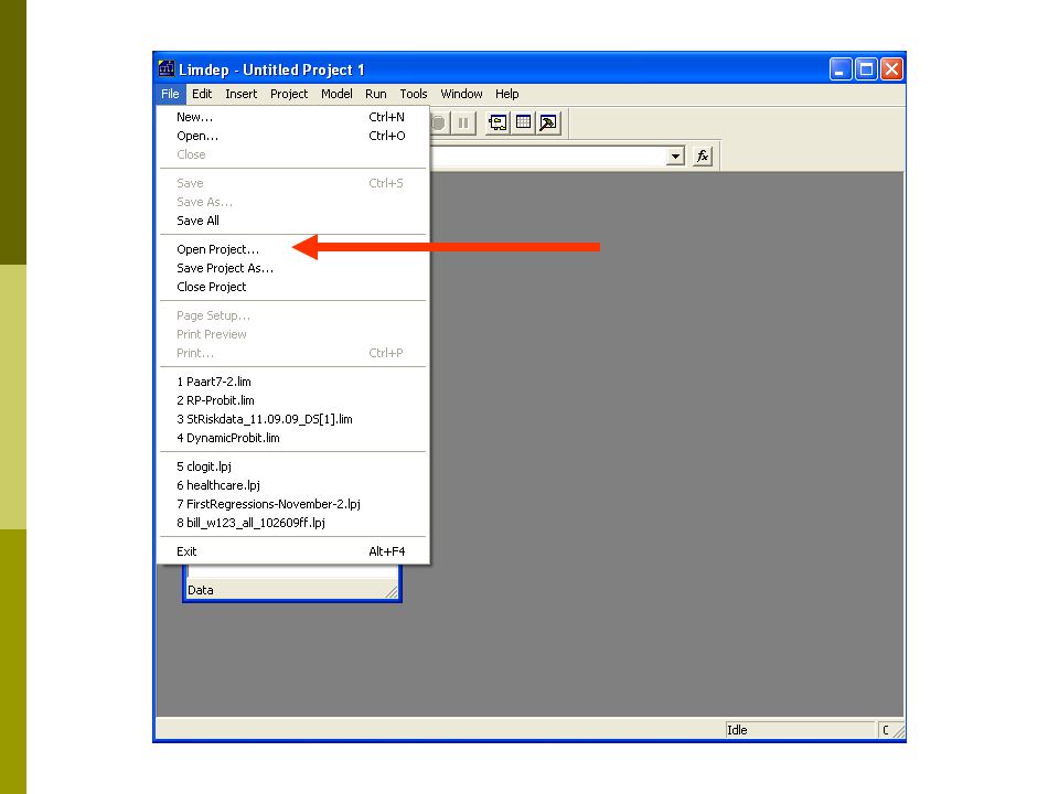
4. Locate file Dairy.lpj Locate file dairy.lpj

5. Project Window Note: Name Sample Size Variables

6. Use File:New/OK for an Editing Window

7. Save Your Work When You Exit

8. Typing Commands in the Editor

9. Important Commands: SAMPLE ; first - last $ Sample ; 1 – 1000 $ Sample ; All $ CREATE ; Variable = transformation $ Create ; LogMilk = Log(Milk) $ Create ; LMC =.5*Log(Milk)*Log(Cows) $ Create ; … any algebraic transformation $

10. Name Conventions CREATE ; name = any result desired $ Name is the name of a new variable No more than 8 characters in a name The first character must be a letter May not contain -,+,*,/. May contain _.

11. Model Command Model ; Lhs = dependent variable ; Rhs = list of independent variables $ Regress ; Lhs = Milk ; Rhs = ONE,Feed,Labor,Land $ ONE requests the constant term Models are REGRESS, PROBIT, POISSON, LOGIT, TOBIT, … and about 100 others. All have the same form.

12. The Go Button

13. “Submitting” Commands One Command Place cursor on that line Press “Go” button More than one command Highlight all lines (like any text editor) Press “Go” button

14. Compute a Regression Sample ; All $ Regress ; Lhs = YIT ; Rhs = One,X1,X2,X3,X4 $ The constant term in the model

16. Project window shows variables Results appear in output window Commands typed in editing window Standard Three Window Operation

17. Model Results Sample ; All $ Regress ; Lhs = YIT ; Rhs =One,X1,X2,X3,X4 ; Res = e ? (Regression with residuals saved) ; Plot Residuals Produces results: Displayed results in output Displayed plot in its own window Variables added to data set Matrices Named Scalars

18. Output Window

19. Residual Plot

20. New Variable Regress;Lhs=Yit;Rhs=One,x1,x2,x3,x4 ; Res = e ; Plot Residuals $ ? We can now manipulate the new ? variable created by the regression. Namelist ; z = Year94,Year95,Year96, Year97,Year98$ Create;esq = e*e / (sumsqdev/nreg) – 1 $ Regress; Lhs = esq ; Rhs=One,z $ Calc ; List ; LMTstHet = nreg*Rsqrd $

21. Saved Matrices B=estimated coefficients and VARB=estimated asymptotic covariance matrix are saved by every model command. Different model estimators save other results as well. Here, we manipulate B and VARB to compute a restricted least squares estimator the hard way. REGRESS ; Lhs = Yit ; Rhs=One,x1,x2,x3,x4 $ NAMELIST ; X = One,x1,x2,x3,x4 $ MATRIX ; R = [0,1,1,1,1] ; q = [1] ; XXI = ; m = R*B – q ; C=R*XXI*R’ ; bstar = B - XXI*R’* *m ; Vbstar=VARB – ssqrd*XXI*R’* *R*XXI $

22. Saved Scalars Model estimates include named scalars. Linear regressions save numerous scalars. Others usually save 3 or 4, such as LOGL, and others. The program on the previous page used SSQRD saved by the regression. The LM test two pages back used NREG (the number of observations used) and RSQRD (the R 2 in the most recent regression).

23. Model Commands Generic form: Model name ; Lhs = dependent variable ; Rhs = independent variables $ Rhs should generally include ONE to request a constant term.

24. Probit Model Command Text Editor Probit ; Lhs = Grade ; Rhs = one,gpa,tuce,psi $ Command builder Load Spector.lpj

25. Model Command