Download presentation
Presentation is loading. Please wait.

1
Chem 300 - Ch 25/#2 Today’s To Do List Binary Solid-Liquid Phase Diagrams Continued (not in text…) Colligative Properties
 Colligative Properties")
2
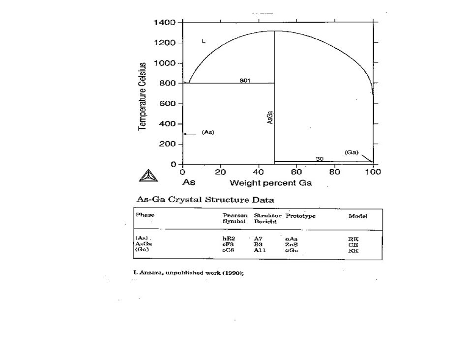
Stable Compound Formation

4
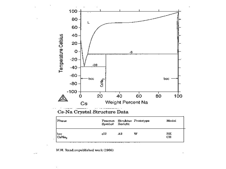
K/Na with incongruent MP & Unstable Compound Formation

10
Colligative Properties l Depends upon only the number of (nonvolatile) solute particles l Independent of solute identity l From colligatus: “depending upon the collection” Vapor pressure lowering Boiling point elevation Freezing point depression Osmotic pressure
 solute particles l Independent of solute identity l From colligatus: depending upon the collection Vapor pressure lowering Boiling point elevation Freezing point depression Osmotic pressure")
11
Basis for Colligativity l Solvent chem potential (μ 1 ) is reduced when solute is added: μ * 1 μ * 1 + RT ln x 1 (“1” is solvent) Since x 1 < 1 ln x 1 < 0 Thus μ 1 (solution) < μ 1 (pure solvent)
 is reduced when solute is added: μ * 1 μ * 1 + RT ln x 1 ( 1 is solvent) Since x 1 < 1 ln x 1 < 0 Thus μ 1 (solution) < μ 1 (pure solvent)")
12
Chemical Potential

13
Vapor Pressure lowering

14
Freezing Point Depression: ΔT fus = K f m l Thermo Condition: At fp: solid solvent in equilib with solvent that’s in soln μ solid 1 (T fus ) = μ soln 1 (T fus ) μ solid 1 = μ * 1 + RT ln a 1 = μ liq 1 + RT ln a 1 l Rearranging: ln a 1 = (μ solid 1 - μ liq 1 )/RT
 = μ soln 1 (T fus ) μ solid 1 = μ * 1 + RT ln a 1 = μ liq 1 + RT ln a 1 l Rearranging: ln a 1 = (μ solid 1 - μ liq 1 )/RT")
15
l Take derivative: ( ln a 1 / T) P, x1 = [(μ solid 1 - μ liq 1 )/RT]/ T Recall Gibbs-Helmholtz equation: [ (μ/T)/ T] P, x1 = - H 1 /T 2 Substitute in above: ( ln a 1 / T) P, x1 = (H liq 1 – H sol 1 )/RT 2 = Δ fus H/RT 2
![l Take derivative: ( ln a 1 / T) P, x1 = [(μ solid 1 - μ liq 1 )/RT]/ T Recall Gibbs-Helmholtz equation: [ (μ/T)/ T] P, x1 = - H 1 /T 2 Substitute in above: ( ln a 1 / T) P, x1 = (H liq 1 – H sol 1 )/RT 2 = Δ fus H/RT 2](http://images.slideplayer.com/11/3278582/slides/slide_15.jpg "l Take derivative: ( ln a 1 / T) P, x1 = [(μ solid 1 - μ liq 1 )/RT]/ T Recall Gibbs-Helmholtz equation: [ (μ/T)/ T] P, x1 = - H 1 /T 2 Substitute in above: ( ln a 1 / T) P, x1 = (H liq 1 – H sol 1 )/RT 2 = Δ fus H/RT 2")
16
( ln a 1 / T) P, x1 = Δ fus H/RT 2 l Integrate between T * fus and T fus : ln a 1 = ƒ (Δ fus H/RT 2 )d T l Since it’s a dilute solution: a 1 ~ x 1 = 1- x 2 ln (1 – x 2 ) ~ - x 2 l Substitute above: - x 2 = (Δ fus H/R)(1/T * fus – 1/T fus )
 P, x1 = Δ fus H/RT 2 l Integrate between T * fus and T fus : ln a 1 = ƒ (Δ fus H/RT 2 )d T l Since it’s a dilute solution: a 1 ~ x 1 = 1- x 2 ln (1 – x 2 ) ~ - x 2 l Substitute above: - x 2 = (Δ fus H/R)(1/T * fus – 1/T fus )")
17
- x 2 = (Δ fus H/R)(T fus - T * fus )/T * fus T fus l Solute lowers the freezing point: T fus < T * fus l Express in molality: x 2 = n 2 /(n 1 + n 2 ) = m/(1000/M 1 + m) But m << 1000/M 1 x 2 ~ M 1 m/1000 (substitute above for x 2 ) l Note: T * fus ~ T fus (T fus - T * fus )/T * fus T fus ~ (T fus - T * fus )/T* 2 fus = - Δ T/T* 2 fus
(T fus - T * fus )/T * fus T fus l Solute lowers the freezing point: T fus < T * fus l Express in molality: x 2 = n 2 /(n 1 + n 2 ) = m/(1000/M 1 + m) But m << 1000/M 1 x 2 ~ M 1 m/1000 (substitute above for x 2 ) l Note: T * fus ~ T fus (T fus - T * fus )/T * fus T fus ~ (T fus - T * fus )/T* 2 fus = - Δ T/T* 2 fus")
18
Substitute! l Δ T fus = K f m Where K f = M 1 R(T * fus ) 2 /(1000Δ fus H) K f is function of solvent only l Similar expression obtained for bp elevation: Δ T vap = K b m Where K b = M 1 R(T * vap ) 2 /(1000Δ vap H) l Compare terms
 2 /(1000Δ fus H) K f is function of solvent only l Similar expression obtained for bp elevation: Δ T vap = K b m Where K b = M 1 R(T * vap ) 2 /(1000Δ vap H) l Compare terms.")
20
Example Comparison l Calc. fp and bp change of 25.0 mass % soln of ethylene glycol (M 1 = 62.1) in H 2 O. l m = n Gly /kg H 2 O = (250/62.1)/(750/10 3 ) = 5.37 l Δ T fus = K f m = (1.86)(5.37) = 10.0 O C l Δ T vap = K b m = (0.52)(5.37) = 2.8 O C
 in H 2 O. l m = n Gly /kg H 2 O = (250/62.1)/(750/10 3 ) = 5.37 l Δ T fus = K f m = (1.86)(5.37) = 10.0 O C l Δ T vap = K b m = (0.52)(5.37) = 2.8 O C.")
21
Osmotic Pressure

22
Example l Calc. Osmotic pressure of previous example at 298 K. l Π = c 2 RT c 2 = 4.0 R = 0.0821 L-atm/mol-K Π = c 2 RT = (4.0)(0.0821)(298) = 97 atm
(0.0821)(298) = 97 atm.")
23
Debye-Hückel Model of Electrolyte Solutions l The Model: An electrically charged ion (q) immersed in a solvent of dielectric constant ε l Experimental Observations: All salt (electrolyte) solutions are nonideal even at low concentrations Equilibrium of any ionic solute is affected by conc. of all ions present.

27
Next Time How to explain the experimental evidence: Debye-Huckel Model of electrolyte solutions

Similar presentations


 = moles of solute liter of solution Dilutions: M 1 x V 1 = M 2 x V 2 Percent by volume.>")

.>")

: mass percentage of the component = X 100% mass.>")


