Download presentation
Presentation is loading. Please wait.

1
Chapter 2 Discrete-time signals and systems
2.1 Discrete-time signals:sequences 2.2 Discrete-time system 2.3 Frequency-domain representation of discrete-time signal and system

2
2.1 Discrete-time signals:sequences
2.1.1 Definition Classification of sequence Basic sequences Period of sequence 2.1.5 Symmetry of sequence Energy of sequence 2.1.7 The basic operations of sequences

3
2.1.1 Definition EXAMPLE Enumerative representation
Function representation

4
Graphical representation
-2 2 4 6 -3 -1 1 5 10 -0.5 0.5 Graphical representation

5
Generate and plot the sequence in MATLAB
x=[1,2,1.2,0,-1,-2,-2.5] stem(n,x, '.') n=0:9 y=0.9.^n.*cos(0.2*pi*n+pi/2) stem(n,y,'.')
 n=0:9. y=0.9.^n.*cos(0.2*pi*n+pi/2) stem(n,y, . )")
6
Sampling the analog waveform
Figure 2.2 EXAMPLE Sampling the analog waveform

7
Display the wav speech signal in ULTRAEDIT

8
Display the wav speech signal in COOLEDIT
The whole waveform Display the wav speech signal in local Blowup

9
2.1.2 Classification of sequence
Right-side Left-side Two-side Finite-length Causal Noncausal

10
2.1.3 Basic sequences 1. Unit sample sequence 2.The unit step sequence
3.The rectangular sequence

11
4. Exponential sequence

13
5. Sinusoidal sequence

14
For convenience, sinusoidal signals are usually expressed by exponential sequences.
The relationship between ω and Ω:

15
Period of sequence

16
Three kinds of period of sequence

17
2.1.5 Symmetry of sequence Conjugate-symmetric sequence
Conjugate-antisymmetric sequence

19
Real sequences can be decomposed into two symmetrical sequences.
EXAMPLE n=[-5:5]; x=[0,0,0,0,0,1,2,3,4,5,6]; xe=(x+fliplr(x))/2 ; xo=(x-fliplr(x))/2; subplot(3,1,1) stem(n,x) subplot(3,1,2) stem(n,xe) subplot(3,1,3) stem(n,xo) Real sequences can be decomposed into two symmetrical sequences.
)/2 ; xo=(x-fliplr(x))/2; subplot(3,1,1) stem(n,x) subplot(3,1,2) stem(n,xe) subplot(3,1,3) stem(n,xo) Real sequences can be decomposed into two symmetrical sequences.")
20
Complex sequences can be decomposed into two symmetrical sequences.
EXAMPLE Complex sequences can be decomposed into two symmetrical sequences. n=[-5:5]; x=zeros(1,11); x((n>=0)&(n<=5))=(1+j).^[0:5] xe=(x+conj(fliplr(x)))/2; xo=(x-conj(fliplr(x)))/2 subplot(3,2,1); stem(n,real(x)) subplot(3,2,2); stem(n,imag(x)) subplot(3,2,3); stem(n,real(xe)) subplot(3,2,4); stem(n,imag(xe)) subplot(3,2,5); stem(n,real(xo)) subplot(3,2,6); stem(n,imag(xo))
; x((n>=0)&(n<=5))=(1+j).^[0:5] xe=(x+conj(fliplr(x)))/2; xo=(x-conj(fliplr(x)))/2. subplot(3,2,1); stem(n,real(x)) subplot(3,2,2); stem(n,imag(x)) subplot(3,2,3); stem(n,real(xe)) subplot(3,2,4); stem(n,imag(xe)) subplot(3,2,5); stem(n,real(xo)) subplot(3,2,6); stem(n,imag(xo))")
21
Energy of sequence

22
2.1.7 The basic operations of sequences

23
Basic operations of sequences

24
Original speech sequences Original music sequence
sequences after scalar multiplication sequences after vector addition sequences after vector multiplication echo

25
The matlab codes on the processions
x=wavread('test1.wav',36000); y=wavread('test2.wav ',36000); z=(x+y)/2.0; wavwrite(z,22050,'test3.wav') y1=y*0.5; wavwrite(y1,22050,'test4.wav') y2=zeros(36000,1); for i=2000:36000 y2(i)=y(i ); end y3=0.6*y+0.4*y2; wavwrite(y3,22050,'test5.wav') w=[0:1/36000:1-1/36000]'; y4=y.*w; wavwrite(y4,22050,'test6.wav') Vector addition realizes composition. scalar multiplication changes the volume. Delay, scalar multiplication and vector addition produce echo. vector multiplication realizes fade-in.
; y=wavread( test2.wav ,36000); z=(x+y)/2.0; wavwrite(z,22050, test3.wav ) y1=y*0.5; wavwrite(y1,22050, test4.wav ) y2=zeros(36000,1); for i=2000: y2(i)=y(i ); end. y3=0.6*y+0.4*y2; wavwrite(y3,22050, test5.wav ) w=[0:1/36000:1-1/36000] ; y4=y.*w; wavwrite(y4,22050, test6.wav ) Vector addition realizes composition. scalar multiplication changes the volume. Delay, scalar multiplication and vector addition produce echo. vector multiplication realizes fade-in.")
26
The matlab codes on the addition of two sequences
EXAMPLE

27
n=[-4:2] ; x=[1,-2,4,6,-5,8,10] ; %x1[n]=x[n+2] n1=n-2; x1=x; %x2[n]=x[n-4] n2=n+4; x2=x; %y[n] m=[min(min(n1),min(n2)): max(max(n1),max(n2))] ; y1=zeros(1,length(m)) ; y2=y1; y1((m>=min(n1))&(m<=max(n1)))=x1;y2((m>=min(n2))&(m<=max(n2)))=x2; y=3*y1+y2; stem(m,y) Output:y =
![n=[-4:2] ; x=[1,-2,4,6,-5,8,10] ; %x1[n]=x[n+2] n1=n-2; x1=x; %x2[n]=x[n-4] n2=n+4; x2=x; %y[n]](http://slideplayer.com/slide/3269643/11/images/27/n%3D%5B-4%3A2%5D+%3B+x%3D%5B1%2C-2%2C4%2C6%2C-5%2C8%2C10%5D+%3B+%25x1%5Bn%5D%3Dx%5Bn%2B2%5D+n1%3Dn-2%3B+x1%3Dx%3B+%25x2%5Bn%5D%3Dx%5Bn-4%5D+n2%3Dn%2B4%3B+x2%3Dx%3B+%25y%5Bn%5D.jpg "m=[min(min(n1),min(n2)): max(max(n1),max(n2))] ; y1=zeros(1,length(m)) ; y2=y1; y1((m>=min(n1))&(m<=max(n1)))=x1;y2((m>=min(n2))&(m<=max(n2)))=x2; y=3*y1+y2; stem(m,y) Output:y =")
28
7.convolution sum: steps:turnover, shift, vector multiplication, addition

29
EXAMPLE nx=0:10; x=0.5.^nx; nh=-1:4; h=ones(1,length(nh))
y=conv(x,h); stem([min(nx)+min(nh):max(nx)+max(nh)],y)
; stem([min(nx)+min(nh):max(nx)+max(nh)],y)")
30
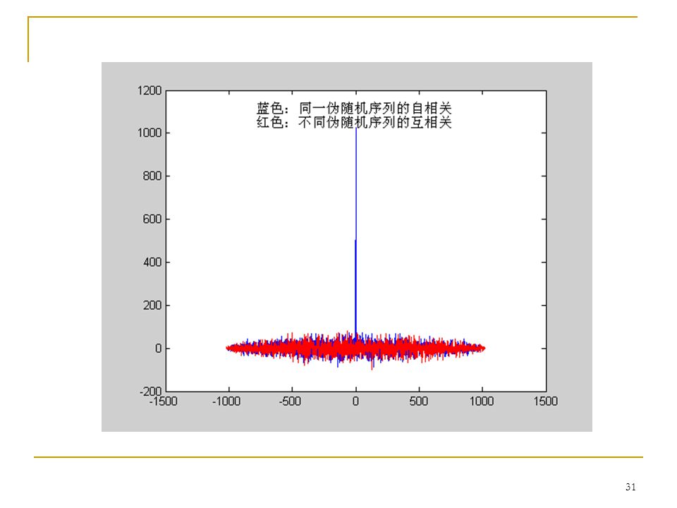
8.crosscorrelation: aotocorrelation:

32
example:correlation detection in digital audio watermark

35
2.1 summary Definition Classification of sequence Basic sequences Period of sequence Symmetry of sequence Energy of sequence 2.1.7 The basic operations of sequences

36
key: convolution requirements:judge the period of sequence ;
calculate convolution with graphical and analytical evaluation . key: convolution

37
2.2 Discrete-time system Definition:input-output description of systems 2.2.2 Classification of discrete-time system Linear time-invariant system(LTI) 2.2.4 Linear constant-coefficient difference equation Direct implementation of discrete-time system
 Linear constant-coefficient difference equation Direct implementation of discrete-time system.")
38
2.2.1 definition:input-output description of systems
the impulse response

39
EXAMPLE

40
2.2.2 classification of discrete-time system
1.Memoryless (static) system the output depends only on the current input. 2.Linear system 3.Time-invariant system: 4.Causal system: the output does not depend on the latter input. 5.Stable system:
 system. the output depends only on the current input. 2.Linear system. 3.Time-invariant system: 4.Causal system: the output does not depend on the latter input. 5.Stable system:")
41
2.2.3 linear time-invariant system(LTI)
How to get h[n] from the input and output:

42
the impulse response in LTI
EXAMPLE

43
Properties of LTI Figure 2.12 h[n]
![Properties of LTI Figure 2.12 h[n]](http://slideplayer.com/slide/3269643/11/images/43/Properties+of+LTI+Figure+2.12+h%5Bn%5D.jpg "Properties of LTI Figure 2.12 h[n]")
44
classification of linear time-invariant system
IIR: h[n]’s length is infinite the latter input the former input FIR must be stable。

45
2.2.4 linear constant-coefficient difference equation
1.relation with input-output description and convolution EXAMPLE For IIR,the latter two are consistent. input-output description convolution description infinite items,unrealizable difference equation description Finite items, realizable

46
EXAMPLE For FIR,the followings are consistent
input-output description and difference equation description (non-recursion) Convolution description Another difference equation description,recursion,lower rank For FIR and IIR,difference equations are not exclusive.
 Convolution description. Another difference equation description,recursion,lower rank. For FIR and IIR,difference equations are not exclusive.")
47
EXAMPLE 2.Recursive computation of difference equations:
For IIR, there needs N initial conditions , then ,the solution is unique. For FIR, there needs no initial conditions. With initial-rest conditions (linear, time invariant, and causal), the solution is unique. EXAMPLE
, the solution is unique. EXAMPLE.")
48
3.computation of difference equations with homogeneous
and particular solution

49
2.2.5. Direct implementation of discrete-time system
EXAMPLE

50
EXAMPLE

51
The matlab codes on the direct realization of LTI
EXAMPLE The matlab codes on the direct realization of LTI B=1; A=[1,-1] n=[0:100]; x=[n>=0]; y=filter(B,A,x); stem(n,y); axis([0,20,0,20])
; stem(n,y); axis([0,20,0,20])")
52
2.2 summary Definition:input-output description of systems 2.2.2 Classification of discrete-time system Linear time-invariant system(LTI) 2.2.4 Linear constant-coefficient difference equation Direct implementation of discrete-time system
 Linear constant-coefficient difference equation Direct implementation of discrete-time system.")
53
judge the type of a system(from the relationship between
keys: judge the type of a system(from the relationship between the input and output, and from h[n] for LTI). the physics meaning of convolution representation for LTI: the output signals are the weighted combination of the input signals, h[n] is the weight。 the similarities and differences between linear constant-coefficient difference equations and convolution representation,recursive computation。 the difference between IIR and FIR: FIR IIR h[n] finite length infinite length y[n]是x[n]的加权 finite items infinite items realization convolution or difference difference , recursion stability stable maybe stable
. the physics meaning of convolution representation for LTI: the output signals are the weighted combination of the input signals, h[n] is the weight。 the similarities and differences between linear constant-coefficient. difference equations and convolution representation,recursive computation。 the difference between IIR and FIR: FIR IIR. h[n] finite length infinite length. y[n]是x[n]的加权 finite items infinite items. realization convolution or difference difference , recursion. stability stable maybe stable.")
54
2.3 frequency-domain representation of discrete-time signal and system
2.3.1 definition of fourier transform frequency response of system 2.3.3 properties of fourier transform

55
EXAMPLE The intuitionistic meaning of frequency-domain representation of signals

56
The intuitionistic meaning of frequency-domain representation of systems

57
The effect of lowpass and highpass filters to image signals
EXAMPLE

58
Frequency-domain analysis of de-noise process through bandstop filter

59
Derivation of Fourier transform

60
2.3.1 definition of fourier transform
arbitrary phase

61
Matlab codes to draw the frequency chart of signals
EXAMPLE subplot(2,2,1); fplot('real(1/(1-0.2*exp(-1*j*w)))',[-2*pi,2*pi]); title('实部') subplot(2,2,2); fplot('imag(1/(1-0.2*exp(-1*j*w)))',[-2*pi ,2*pi]); title('虚部') subplot(2,2,3); fplot('abs(1/(1-0.2*exp(-1*j*w)))',[-2*pi,2*pi]); title('幅度') subplot(2,2,4); fplot('angle(1/(1-0.2*exp(-1*j*w)))',[-2*pi,2*pi]); title('相位') Matlab codes to draw the frequency chart of signals
; fplot( real(1/(1-0.2*exp(-1*j*w))) ,[-2*pi,2*pi]); title( 实部 ) subplot(2,2,2); fplot( imag(1/(1-0.2*exp(-1*j*w))) ,[-2*pi ,2*pi]); title( 虚部 ) subplot(2,2,3); fplot( abs(1/(1-0.2*exp(-1*j*w))) ,[-2*pi,2*pi]); title( 幅度 ) subplot(2,2,4); fplot( angle(1/(1-0.2*exp(-1*j*w))) ,[-2*pi,2*pi]); title( 相位 ) Matlab codes to draw the frequency chart of signals.")
62
Fourier transforms of non-absolutely summable or non-square summable signals
EXAMPLE EXAMPLE

63
2.3.2 frequency response of system

64
Ideal filter in frequency and time domain
EXAMPLE

65
Matlab codes to draw the frequency response of a system
EXAMPLE h=[1,0,0,0,0,0,0,0,0,0.5] freqz(h,1)
")
66
Eigenfunction and steady-state response:
Steady-state response transient response

67
Figure 2.20 causal FIR system acts on causal signal
Causal and stable IIR system acts on causal signal Figure 2.20

68
example of steady-state response
Sin(0.1*pi*n) h[n]=[1,1,1,1,1,1,1,1,1,1]/4 B=[1,0,1,0,1];A=[1,0.81,0.81,0.81]
 h[n]=[1,1,1,1,1,1,1,1,1,1]/4. B=[1,0,1,0,1];A=[1,0.81,0.81,0.81]")
69
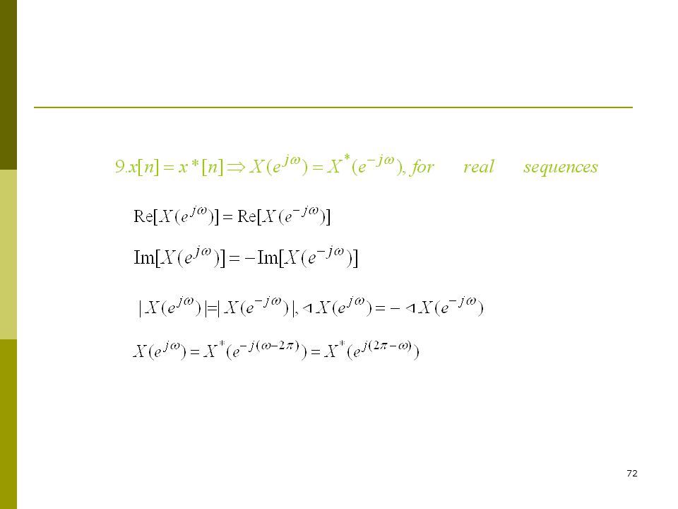
2.3.3 properties of fourier transform

73
2.3 summary 2.3.1 definition of fourier transform frequency response of system 2.3.3 properties of fourier transform requirements:calculation of fourier transforms steady-state response linearity time shifting frequency shifting the convolution theorem windowing theorem Parseval’s theorem symmetry properties

74
exercises: 2.35 2.45 2.57 Keys and difficulties:
the convolution theorem; the frequency spectrum of a real sequence is conjugate symmetric; the frequency spectrum of a conjugate symmetric sequence is a real function. exercises:

Similar presentations


,>")


![Discrete Time Periodic Signals A discrete time signal x[n] is periodic with period N if and only if for all n. Definition: Meaning: a periodic signal keeps.](/18/5705308/big_thumb.jpg "Discrete Time Periodic Signals A discrete time signal x[n] is periodic with period N if and only if for all n. Definition: Meaning: a periodic signal keeps.>")


