1. Microsoft Excel Manual 1 By Pradeep velugoti Lakshman Tallam

2. Overview:  Worksheet title.  Calculating Sum and Average.  Generating Multiple Values.  Changing Cell Style.  Adjusting Column Width.  Inserting Rows and Columns.  Formatting Cells.  Inserting Graphs.

3. What is a Spreadsheet?  A spreadsheet is the computer equivalent of a paper ledger sheet. It consists of a grid made from columns and rows. Columns are alphabetically labeled and rows are numerically labeled. The junction of a Column and row is referred to as a Cell. A cell is referenced by it column and row reference, for example A15, G47, U76

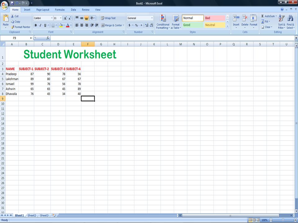
4. To Enter the Worksheet Title  Click cell A1 to make cell A1 the active cell.  Type the title of the worksheet.  For example “Student Worksheet”.  And then point to the enter button in the formula box and click on it to complete the entry.  Now select the cells from A1 to H1, Click on the Merge and Center button in the alignment group to center the title.

5. Cancel Box Enter Box Formula Bar

6. Click on Merge and Center Button

8.  Now lets enter some data in the spreadsheet.  There are four basic types of data you can enter into a cell.  Labels or Characters  Values or numeric  Formulas cell references and math functions For example, A1+B1+C1+D1+E1  Functions that are built in Formulas For example SUM(A1:E1)

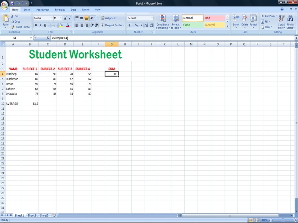
10. Summing a Column of Numbers  Click cell G4 to make it the active cell and then point to the SUM button on the Ribbon.  Click the Sum button on the Ribbon to display =SUM(B4:E4) in the formula bar and in the active cell G4.  Click the Enter box in the formula bar to enter the sum of all subjects of a student.  Select cell G4 to display the SUM function assigned to cell G4 in the formula bar.

11. Click on the SUM button

12. Change the cell range from F4 to E4 and hit ENTER button.

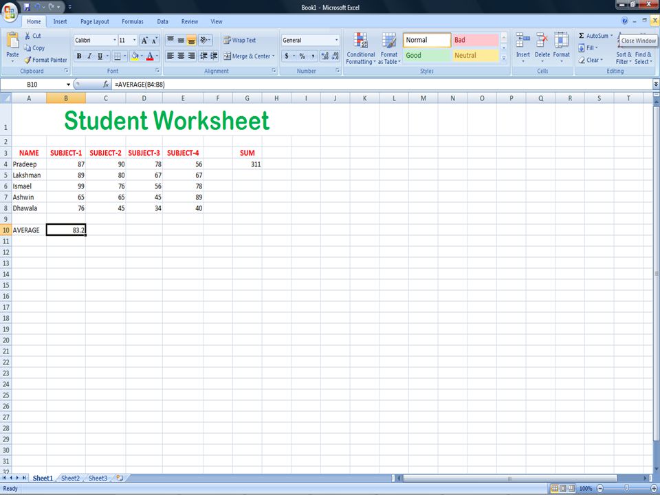
13. Calculating the Average  Click cell B10 to make it the active cell and then point to the AVERAGE button on the Ribbon.  Click the AVERAGE button on the Ribbon to display =AVERAGE(B4:B8) in the formula bar and in the active cell B10.  Click the Enter box in the formula bar to enter the average of a subject.  Select cell B10 to display the AVERAGE function assigned to cell B10 in the formula bar.

14. Click on the AVERAGE function and hit ENTER button.

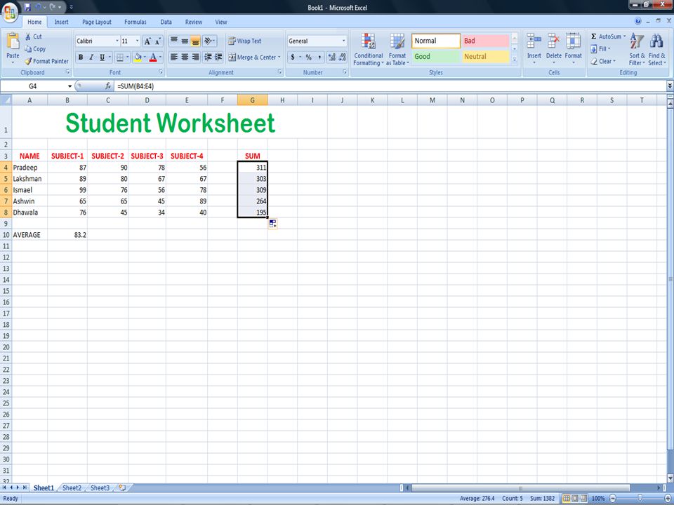
16. Determining Multiple Totals at the Same Time  Click cell G4 to make it the active cell.  With the mouse pointer in cell G4 and in the shape of a block plus sign, drag the mouse pointer down to cell G8.  The same function of G4 will be applied to all the cells till G8.

19. Changing a Cell Style  Click cell A3 to make cell A3 the active cell.  Click the Cell Styles button on the Ribbon to display the Cell Styles gallery.  Point to the Title cell style in the Titles and Headings area of the Cell Styles gallery to see a live preview of the cell style in cell A3.  Click the Title cell style to apply the cell style to cell A3.

20. Adjusting Column Width  Point to the boundary on the right side of the column A heading above row 1 to change the mouse pointer to a split double arrow.  Double-click on the boundary to adjust the width of column A to the width of the largest item in the column.

21. Inserting New Rows and Columns  Click on the Insert Button in the Cells group and select Insert Cells to insert a new row or a column.

22. Click on Insert Cells and then choose to insert an entire row or a column

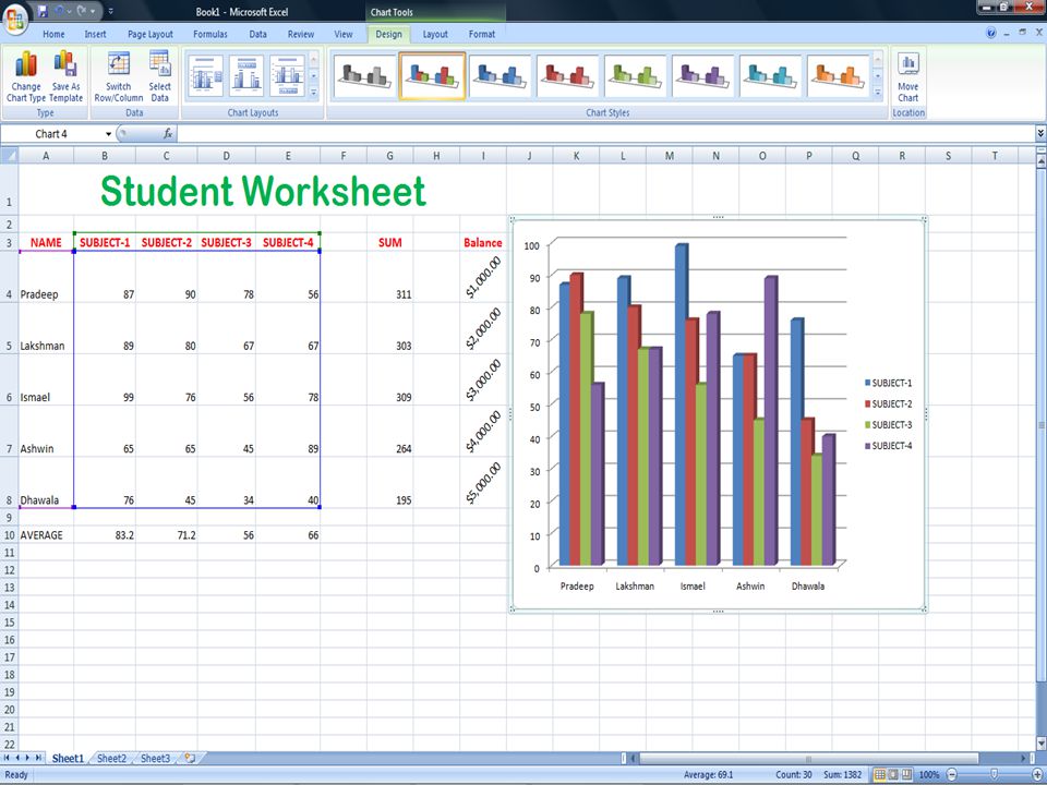
23. Inserting Graphs  Select the cells from A3 to E8.  Click on the Insert tab and then choose the chart type in the charts group.  To switch the row and column in the chart, Right click on the chart and then select the option “select data”.  Then click on the button “Switch Row/Column”.

26. Click on Switch Row/Column

28. Formatting Cells  Now lets include one more field in the worksheet in the name of “Currency” in cell I3 and then enter some data in number format in the cells below that.  We would like that entered data to be displayed in currency format.  For that purpose select all the cells from I4 to I8, Right click on those cells and select Format Cells.

29.  In the Number tab, change the category from general to currency. We can even increase or decrease the decimal points of the currency.  We can also include a ‘$’ sign for the currency data.  In the alignment tab, we can change the orientation of the text by changing the angle of the text.  To avoid the text entered into the selected cell from overlapping into another cell, select the wrap text option form the alignment group.

31. Change the angle of the text